VOLUME 40, ARTICLE 19, PAGES 503
-
532
PUBLISHED 8 MARCH 2019
https://www.demographic-research.org/Volumes/Vol40/19/ DOI: 10.4054/DemRes.2019.40.19
Research Article
Combining population projections with
quasi-likelihood models: A new way to predict cancer
incidence and cancer mortality in Austria up to
2030
Johannes Klotz
Monika Hackl
Markus Schwab
Alexander Hanika
Daniela Haluza
© 2019 Johannes Klotz et al.
This open-access work is published under the terms of the Creative Commons Attribution 3.0 Germany (CC BY 3.0 DE), which permits use, reproduction, and distribution in any medium, provided the original author(s) and source are given credit.
1 Introduction 504
2 Materials and methods 505
2.1 Terminology 505
2.2 Data 506
2.2.1 Primary population projection 506
2.2.2 Austrian National Cancer Registry 506
2.2.3 Austrian Cause of Death Statistics 507
2.2.4 Tumor sites 508
2.3 Forecasting cancer incidence and cancer death rates 508 2.3.1 Quasi-Poisson regression with offset parameter 509
2.3.2 Regressors used in all models 510
2.3.3 Special regressors used in some models 512
2.3.4 Software implementation and prediction 513
2.4 Sensitivity analysis: Constant rates scenario 514
3 Results 514
3.1 Estimated regression parameters 514
3.1.1 Example: Incidence of head and neck cancer for males 515
3.1.2 Estimated trend parameters 516
3.2 Predicted future cancer counts and age-standardized rates 517
3.2.1 Aggregate (all-site) outcomes 517
3.2.2 Site-specific outcomes 520
4 Discussion 521
4.1 Summary and comparison with international findings 521
4.2 Uncertainty in our model predictions 523
4.2.1 Reliability 523
4.2.2 Validity 524
5 Conclusion 526
6 Funding 526
7 Acknowledgements 526
References 527
Combining population projections with quasi-likelihood models:
A new way to predict cancer incidence and cancer mortality in
Austria up to 2030
Johannes Klotz1‡ Monika Hackl1‡ Markus Schwab2 Alexander Hanika1
Daniela Haluza2*
Abstract
BACKGROUND
The current demographic changes with a shift toward older ages contribute to more cancer cases in the next decades in Western countries. Thus, forecasting the demand for expected healthcare services and expenditures is relevant for planning purposes and resource allocation.
OBJECTIVE
In this study, we provide a new method to estimate future numbers of cancer cases (newly diagnosed cancers and cancer deaths) using Austrian data.
METHODS
We used 1983–2009 data to estimate cancer burden trends using quasi-Poisson regression models, which we then applied to official population projections up to 2030. Specific regression models were estimated for cancer incidence and mortality, disaggregated by sex and 16 tumor sites.
RESULTS
The absolute number of cancer cases increased continuously during the last decades in Austria. The trend will also continue in the near future, as the number of newly diagnosed cancers and cancer deaths will increase by +14% and +16% between 2009 and 2030. Age-standardized individual risk of being newly diagnosed with or die from
1
Statistics Austria, Vienna, Austria. 2
Department of Environmental Health, Center for Public Health, Medical University of Vienna, Austria. *
cancer will be substantially lower in 2030 compared to 2009 (–14% and –16%, respectively).
CONTRIBUTION
Our novel method combining population projections with quasi-likelihood models found a falling individual risk for cancer burden in the Austrian population. However, the absolute number of new cancer cases and deaths will increase due to the aging of the population. These estimates should be considered when planning future healthcare demands.
1. Introduction
Health planners rely on cancer predictions to optimize allocation of limited resources for primary prevention, screening, treatment, rehabilitation, and palliative care. The most common types of cancer are lifestyle-related, and thus largely preventable (Anand et al. 2008). From a public health perspective, predictions show the effect of health promotion and cancer prevention programs aimed at reducing the burden of cancer in the targeted population (Moller et al. 2007). Changes in population size and structure and changes in individual cancer risk are relevant parameters for anticipating trends in future cancer cases (Bray and Moller 2006). Population-wise changes also depend on immigration and emigration. Given the current demographic trends toward increasing life expectancy, low birth rate, and the baby boomer generation advancing in years, the utmost important time-related variable influencing cancer trends is age. An aging organism accumulates exposure to carcinogens (external factors) and also cancer-inducing spontaneous cell mutations and genetic instability (internal factors) (Finkel, Serrano, and Blasco 2007).
Future changes in disease rates are generally estimated on the basis of those observed in the past. In that respect, a crucial question is to what extent past developments were shaped by the evolution of risk factors (e.g., smoking), population characteristics (e.g., age structure, migrant population), measurement problems (e.g., under-registration of events), and other relevant issues (e.g., outcome-related latency periods), for these influences may evolve differently in the future. A model that fits the data does not necessarily have to provide successful predictions, but a prediction from a model that does not fit past observations is rarely adequately predictive (Valls et al. 2015).
more complex models incorporate the past components of change due to age, period, and birth cohort effects (O’Brien 2000; Olsen, Parkin, and Sasieni 2008). In the United Kingdom, as an example, previous studies have employed such models to generate cancer mortality projections up to 2025 (Olsen, Parkin, and Sasieni 2008; Mistry et al. 2011) and cancer incidence projections up to 2020 (Moller et al. 2007).
In Austria, the proportion of the population aged 65+ will grow from 18% in 2012 to 24% by 2030, mainly as a result of the aging of the baby-boom generation born in the late 1950s and early 1960s. This means that Austria will face significant population aging in the near future. Consistent and accurate data as found in Austrian databases are vital for estimating trends in cancer incidence based on cancer registration data (Doll and Peto 1981). So far, estimates of the corresponding future burden of cancer in terms of numbers of cases are lacking. Thus, we aimed at predicting future cancer cases in Austria for 2010–2030 using 1983–2009 data from the Austrian National Cancer Registry, the Austrian Causes of Death Statistics, and the Population Projections by Statistics Austria. For that purpose, we introduced a new statistical approach of a secondary population projection to predict cancer incidence and cancer mortality of all tumor sites accounting for the available Austrian data.
2. Materials and methods
2.1 Terminology
2.2 Data
2.2.1 Primary population projection
Statistics Austria, the Austrian national statistical institute, regularly publishes long-run cohort-component population projections by sex, age, and nine NUTS-2 regions, i.e., Burgenland, Carinthia, Lower Austria, Upper Austria, Salzburg, Styria, Tyrol, Vorarlberg, and Vienna (Statistik Austria 2014). Several variants are published, combining high, medium, and low-level assumptions on future fertility, mortality, and migration. The main variant of population projections combines medium assumptions on each demographic process, for it is understood to be the most likely future path of the Austrian population. So this variant assumes a slight increase in period fertility, a continuous increase in life expectancy, and enduring positive net migration over the next decades. Details on assumptions and methods are described elsewhere (Hanika 2013). Herein, we used the main variant of the 2013 generation of population projection to 2030, as uncertainty of the forecasted cancer incidence and mortality rates with which the primary population projection is combined would increase for later years – not so much in terms of statistical prediction error, but regarding the stability of structural relationships in the regression specifications. The most important outcome of the primary population projection is a substantial increase in the elderly population (65+ years) from just over 1.5 million in 2013 to almost 2.2 million in 2030. Besides increasing life expectancy, the main driver of this demographic change is the aging of the baby boomer cohorts.
2.2.2 Austrian National Cancer Registry
The Austrian National Cancer Registry is a population-based cancer registry that provides data on cancer incidence, survival, and prevalence. Data has been published since the year of diagnosis 1983 because, since then, individual records can be linked to the Austrian Cause of Death Statistics, which is essential for completeness of registration. Reporting newly diagnosed cancer cases to the Austrian National Cancer Registry is mandatory by law for all Austrian hospitals.
stages. Cancer incidence data is enriched by death certificate only (DCO) cases, i.e., when the death certificate of a deceased person who was not registered in the cancer registry indicates a tumor disease. The tumor information in the database of the Austrian National Cancer Registry is coded according to International Classification of Diseases O-3 (ICD-O-3). When moving to a new classification, e.g., from ICD-O-2 to ICD-O-3, the whole database is recoded using the free software CanReg5 for cancer registry data input, storage, and analysis (CanReg5 2016). ICD-10 codes are added to the data when extracted from the database by using this multi-user, multi-platform, open-source tool produced by the International Agency for Research on Cancer in collaboration with the International Association of Cancer Registries (IARC/IACR).
Currently, there are about 38,000 newly diagnosed cancer cases per year in Austria, thereof 20,000 among men and 18,000 among women. The most frequently diagnosed cancers are prostate cancer, lung cancer, and colon cancer among males, and breast cancer, lung cancer, and colon cancer among females. Around 9% of the total incidence count is DCO cases, with some variation between NUTS-2 regions.
2.2.3 Austrian Cause of Death Statistics
Since 1945, the collection of death records (including cause of death) in Austria is based on administrative records of 1,400 civil registry offices, which in turn are based on reports from hospitals and medical examiners who deliver medical and demographic characteristics and information on cause of death. Death registration is mandatory by law and virtually complete, although deaths of Austrian residents dying abroad were insufficiently covered before 2009.
The Austrian death certificate contains – in addition to the information on the immediate cause and the underlying cause of death – information on the course of the diseases. In Austria, mono-causal causes of death are recorded, which means that only the underlying cause is coded by a trained team according to ICD-10. The death certificate can be issued only by officially appointed physicians, pathologists, or coroners. Therefore, the quality of the cause of death statistics depends on the quality of the data provided by medical doctors. In most cases clinical diagnoses are used to describe the cause of death. An autopsy is performed in about one-tenth of all deaths.
2.2.4 Tumor sites
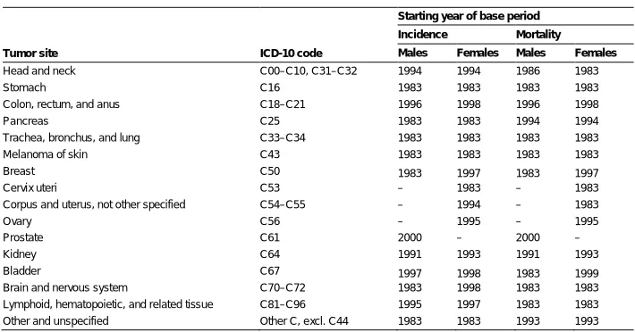
Cancer is partitioned into 16 tumor sites for this projection. Out of the 16 tumor sites, 13 are applicable to males and 15 to females. Details on the disaggregation, including ICD-10 codes, are given in Table 1. Traditionally, head and neck cancers were classified as ICD-10 C00–C10 and C31–C32 in Austria, and this was still the case when we queried our data. Just recently, the definition of head and neck cancers was changed to C00–C14 to enhance international comparability of the data, which however did not influence the predictions presented herein. We forecast cancer incidence and cancer mortality rates for each sex and tumor site, so in total we estimate (13 + 15) × 2 = 56 models.
Table 1: Tumor sites, ICD-10-codes and starting years of base periods
Tumor site ICD-10 code
Starting year of base period Incidence Mortality Males Females Males Females
Head and neck C00–C10, C31–C32 1994 1994 1986 1983 Stomach C16 1983 1983 1983 1983 Colon, rectum, and anus C18–C21 1996 1998 1996 1998 Pancreas C25 1983 1983 1994 1994 Trachea, bronchus, and lung C33–C34 1983 1983 1983 1983 Melanoma of skin C43 1983 1983 1983 1983 Breast C50 1983 1997 1983 1997 Cervix uteri C53 – 1983 – 1983 Corpus and uterus, not other specified C54–C55 – 1994 – 1983
Ovary C56 – 1995 – 1995
Prostate C61 2000 – 2000 –
Kidney C64 1991 1993 1991 1993 Bladder C67 1997 1998 1983 1999 Brain and nervous system C70–C72 1983 1998 1983 1983 Lymphoid, hematopoietic, and related tissue C81–C96 1995 1997 1983 1983 Other and unspecified Other C, excl. C44 1983 1983 1993 1993
Source: Own calculations.
Note: The end year of each base period is 2009.
2.3 Forecasting cancer incidence and cancer death rates
model estimation and then applied estimated parameters to the calendar years 2010– 2030 for predictions.
2.3.1 Quasi-Poisson regression with offset parameter
All 56 models conditional on sex, tumor site, and incidence/mortality are quasi-Poisson regression models with exponential mean function, or equivalently, log-link function (McCullagh and Nelder 1989; Cameron and Trivedi 1998).
In a general sense, denote byP the size of the risk population (i.e., the person-years lived during a calendar year), by Y the cancer count of interest (either newly diagnosed cancer cases or cancer deaths), byt the calendar year, and byx a column vector of other explanatory variables such as age group or region (details are given below). Then our model (1) assumes that
( | , , ) ≔ = × exp( + ), (1)
withθ andβ the parameters to be estimated.
The exponential mean function specification means that regression parameters are semi-elasticities, implying that an increase of time by one calendar year means a constant percentage change in the expected value ofY, holding other factors constant. This assumption is natural for count data, which also guarantees non-negative predictions. The mean function specification was checked by graphical inspection of residuals.
In model (1) population, sizeP is an offset variable. The ratioY/P denotes the rate of cancer incidence or mortality. For the years 1983–2012, population sizes were known from Austrian population statistics data. For the years 2013–2030, the projected values obtained by the primary population projection as described above were applied. As mentioned before, cancer incidence refers not only to first-time tumor diseases, but the same person may be diagnosed several times with different tumor diseases. So, in any given year, the entire Austrian (observed or projected) population is at risk of being newly diagnosed or dying from cancer.
account for overdispersion. A straightforward technique is quasi-Poisson regression, which is an instance of Generalized Linear Models (McCullagh and Nelder 1989; Cameron and Trivedi 1998). Quasi-Poisson regression assumes that
( | , , )= × , (2)
withφ the dispersion parameter. A value greater than 1 means overdispersion.
So the conditional variance of the cancer count of interest is not identical but proportional to its conditional expectation. In quasi-likelihood terms, the nominal Poisson variance μ accounts for pure chance fluctuations, whereas the dispersion parameter φ accounts for unobserved heterogeneity in the conditional mean (Winkelmann 2010).
2.3.2 Regressors used in all models
All 56 regression models included a time trend operationalized by the calendar year. The Austrian National Cancer Registry started to publish data for the year of diagnosis 1983, and 2009 was considered the latest year of sufficient data quality (completeness of registration). We estimated the trend parameter from 1983–2009 and then applied the estimated parameter to the 2010–2030 period. However, graphical (human eye) inspection of age-standardized rates revealed structural breaks within the 1983–2009 period for some tumor sites. For example, female breast cancer incidence increased sharply until the mid-1990s but has remained rather constant since. So the starting year of the base period was in some instances chosen later than 1983, as shown in Table 1. We specified 2000 as the latest possible starting year of the base period so that any base period covers at least ten calendar years, and all base periods end in 2009.
Figure 1: Age profiles of incidence and mortality of selected cancers
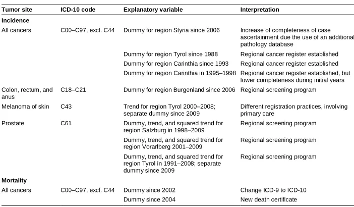
Table 2: Special regressors used in some models
Tumor site ICD-10 code Explanatory variable Interpretation Incidence
All cancers C00–C97, excl. C44 Dummy for region Styria since 2006 Increase of completeness of case ascertainment due the use of an additional pathology database
Dummy for region Tyrol since 1988 Regional cancer register established Dummy for region Carinthia since 1993 Regional cancer register established Dummy for region Carinthia in 1995–1998 Regional cancer register established, but
lower completeness during initial years Colon, rectum, and
anus
C18–C21 Dummy for region Burgenland since 2006 Regional screening program
Melanoma of skin C43 Trend for region Tyrol 2000–2008; separate dummy since 2009
Different registration practices, involving primary care
Prostate C61 Dummy, trend, and squared trend for region Salzburg in 1998–2009
Regional screening program
Dummy, trend, and squared trend for region Vorarlberg 2001–2009
Regional screening program
Dummy, trend, and squared trend for region Tyrol in 1991–2008; separate dummy since 2009
Regional screening program
Mortality
All cancers C00–C97, excl. C44 Dummy since 2002 Change ICD-9 to ICD-10 Dummy since 2004 New death certificate
2.3.3 Special regressors used in some models
The data available for the base period contained the reported number of cancer cases (incidence and mortality) for a specific site. Changes in reporting behavior during the base period thus influence observed trends. To give an example, introducing regional cancer registries clearly increased completeness of ascertained cases for reported regional cancer incidence rates (Hackl and Waldhoer 2013). A challenge in forecasting incidence and mortality rates is to disentangle such data artifacts from real trends, for only the latter should be used in forecasts. Regarding cancer incidence, we identified several influences on reporting behavior in the 1983–2009 period. In particular, two regions introduced regional cancer registries with substantial impact on completeness, and four regions introduced regional screening programs for specific tumor sites.
Predictors that were included in only some of the 56 models are given in Table 2. We modeled the presence of a regional cancer registry by a dummy variable, assuming that its effect on the measured cancer incidence count is essentially a one-shot shift in completeness (except in one instance, where we also accounted for some initial problems with the regional registry).
incidence bulk when tumors are diagnosed earlier than before. Ultimately, a screening program should merely increase completeness. We therefore accounted for both short-run and long-short-run effects of screening programs by including a quadratic trend in the first years of the program (except in one instance, where the screening program only started in 2006) and a dummy variable for the entire period of the program.
Regarding cancer mortality, the change in ICD version from revision 9 to revision 10 and the use of a new death certificate could matter for some tumor sites in particular. So we included dummy variables for the years after 2001 (change in ICD) and for the years after 2003 (new death certificate).
2.3.4 Software implementation and prediction
Population data (observed for 1983–2012, projected for 2013–2030), cancer incidence counts from the Austrian National Cancer Registry (date of query: 17 October 2013), and cancer death counts from the Austrian Cause of Death Statistics were processed in SAS, Version 9.3 (SAS Institute Inc., Cary, North Carolina, USA). The statistical models (1) were estimated by the GENMOD procedure. Dispersion parameters in equations (2) were estimated by dividing the generalized chi-square statistics by its degrees of freedom (Cameron and Trivedi 1998).
Estimated regression parameters and were applied to projected population figures to forecast future cancer incidence and cancer death counts:
= × exp + . (3)
Note that predicted counts are generally not integer-valued.
To obtain overall (all-site) predictions of future cancer incidence and cancer death counts, we summed up the site-specific predictions over all sites.
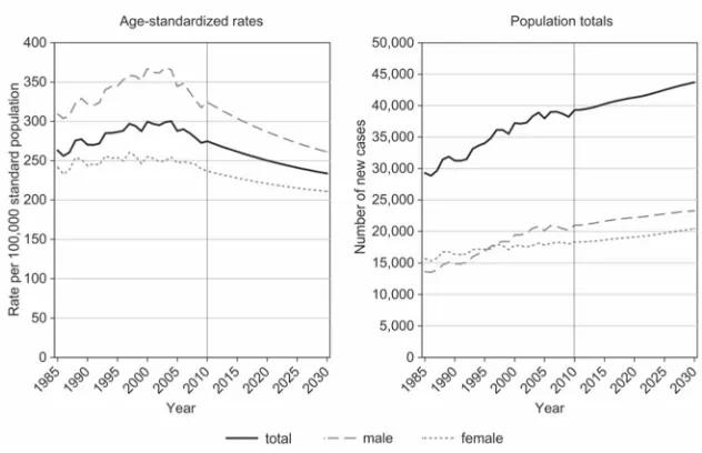
Absolute values of future cancer incidence and death counts are important for healthcare planning and resource allocations. Besides such aggregate outcomes, from a Public Health perspective it is also important to predict the evolution of individual risks. For that purpose we computed age-standardized rates of cancer incidence and mortality by direct age standardization based on the WHO World 2000–2025 Standard Population (Ahmad et al. 2001).
2.4 Sensitivity analysis: Constant rates scenario
Given the projected substantial increase in the elderly population in the coming decades, aggregate cancer counts in the population might increase despite falling individual risk if the decline in individual risk is numerically over-compensated by population aging. An interesting question in that respect is the effect of population aging alone, i.e., how future cancer incidence and mortality counts would evolve if individual risk remained constant in the future. For that purpose, we made an alternative prediction based on a constant rates scenario that keeps age-specific cancer incidence, cancer mortality, and all-cause mortality rates constant over the entire prediction period. We used a three-year average 2008–2010 to minimize random fluctuations. The deviation between our prediction (3) and the values obtained by the alternative constant rates scenario then indicate to what extent changes in risk behavior, as well as medical and social progress (which are implicitly included in the time-trend parameters), alter the future evolution of cancer counts that would result purely from age structure changes.
3. Results
3.1 Estimated regression parameters
Table 3: Estimated regression model for male head and neck cancer incidence
Predictor Estimated maximum quasi-likelihood parameter
Estimated asymptotic standard error P-value
Estimated incidence rate ratio
Logged person-years lived 1
Intercept –7.26 0.08 ***
Age group
0–34 years –4.88 0.12 *** 0.01 35–44 years –1.90 0.07 *** 0.15 45–54 years –0.34 0.07 *** 0.71 55–64 years 0.17 0.06 ** 1.18 65–74 years 0.14 0.07 * 1.15 75–84 years 0.05 0.07 1.06 85 years and older (reference) 0 – 1
NUTS-2 region
Burgenland 0.25 0.05 *** 1.29 Carinthia 0.10 0.05 * 1.10 Lower Austria –0.03 0.03 0.97 Upper Austria –0.04 0.03 0.96
Salzburg –0.07 0.05 0.93
Styria –0.07 0.04 * 0.93
Tyrol 0.14 0.04 *** 1.15
Vorarlberg 0.06 0.05 1.07
Vienna (reference) 0 – 1
Calendar year (time trend) –0.02 0.00 *** 0.98 Indicator: Styria since 2006 0.26 0.06 *** 1.29 Indicator: Carinthia 1995–1998 –0.05 0.08 0.95
Note: * p<0.05, ** p<0.01, *** p<0.001. The intercept parameter depends on the coding of the other parameters, so its p-value has no meaning. The quasi-likelihood dispersion parameter for this model was estimated 1.10.
3.1.1 Example: Incidence of head and neck cancer for males
Table 3 contains the estimated regression parameters and their estimated standard errors of model (1) for male incidence of head and neck cancer (ICD-10 C00–C10 and C31– C32) of the base period from 1994 to 2009. Logged population size (person-years lived) was included as an offset parameter, i.e., its regression coefficient was fixed at 1. The estimated trend parameter is –0.0152, meaning that holding other factors constant, male head and neck cancer incidence is estimated to decline by around 1.5% annually. The parameters in the table refer to the logged cancer incidence count. If the estimated parameter is close to zero, then the linear change in the logged count approximates the proportional change in the proper count. The standard error indicates that this trend is significantly different from zero (p < 0.001), i.e., conditional on all other covariates, male head and neck cancer incidence risk did actually decline in the 1994–2009 period.
smaller, although without statistically significant difference from the maximum. To account for the observed regional variation in incidence risk, we included two special regressors in this model. The fixed effect for Styria from calendar year 2006 onward indicates a 29% increase of completeness of case ascertainment due to an additional pathology database, and an effect for Carinthia in 1995–1998 indicates a 5% underestimation in the initial years of the regional cancer registry. The dispersion parameter is estimated at 1.10, indicating some unobserved heterogeneity in our data.
3.1.2 Estimated trend parameters
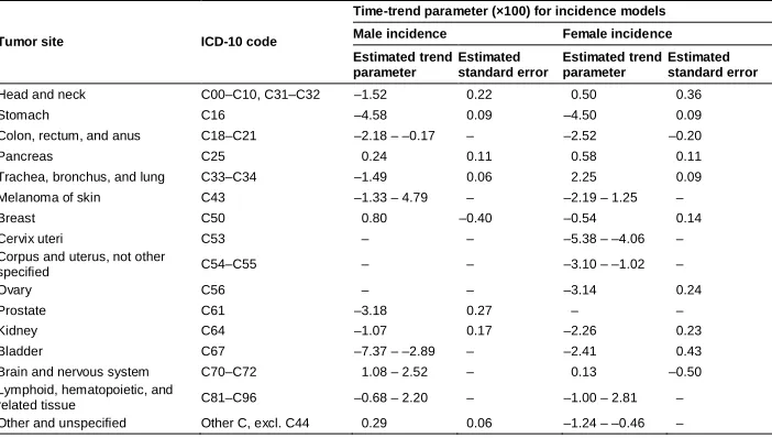
Tables 4 and 5 show the estimated trend parameters for all 56 models, multiplied by 100. We present estimated trend parameters and standard errors for the models where a common time-trend parameter was applied to all nine NUTS-2 regions (like the exemplary model in Table 3). We further present the range of estimated parameters (i.e., minimum to maximum) for the models where different trend parameters were estimated for different (groups of) NUTS-2 regions.
Table 4: Estimated time-trend parameters (×100) for cancer incidence models
Tumor site ICD-10 code
Time-trend parameter (×100) for incidence models Male incidence Female incidence Estimated trend
parameter
Estimated standard error
Estimated trend parameter
Estimated standard error
Head and neck C00–C10, C31–C32 –1.52 0.22 0.50 0.36 Stomach C16 –4.58 0.09 –4.50 0.09 Colon, rectum, and anus C18–C21 –2.18 – –0.17 – –2.52 –0.20 Pancreas C25 0.24 0.11 0.58 0.11 Trachea, bronchus, and lung C33–C34 –1.49 0.06 2.25 0.09 Melanoma of skin C43 –1.33 – 4.79 – –2.19 – 1.25 – Breast C50 0.80 –0.40 –0.54 0.14 Cervix uteri C53 – – –5.38 – –4.06 – Corpus and uterus, not other
specified C54–C55 – – –3.10 – –1.02 –
Ovary C56 – – –3.14 0.24
Prostate C61 –3.18 0.27 – – Kidney C64 –1.07 0.17 –2.26 0.23 Bladder C67 –7.37 – –2.89 – –2.41 0.43 Brain and nervous system C70–C72 1.08 – 2.52 – 0.13 –0.50 Lymphoid, hematopoietic, and
related tissue C81–C96 –0.68 – 2.20 – –1.00 – 2.81 – Other and unspecified Other C, excl. C44 0.29 0.06 –1.24 – –0.46 –
In accordance with decreasing all-site age-standardized rates, estimated trend parameters were negative for most tumor sites. Stomach cancer incidence and mortality rates for both males and females are forecast to decrease by 4% to 5% annually, controlling for age, region, and specific dummy variables. Male prostate cancer incidence and mortality risks are forecast to decline by around 3% annually. For most tumor sites, incidence and mortality trend parameters point in a similar direction, although they may be of different magnitude. Regarding colon cancer for example, the incidence rate is forecast to decline by around 2%, but the mortality rate by around 4% per year, implying that the mortality/incidence ratio is predicted to decline. For female breast cancer, we forecast an annual decline in incidence risk by 0.5% and in mortality risk by 1.4%.
A single trend parameter for all regions was estimated in 42 models and regionally different trends in 14 models. Regional variation in trends was found more often for incidence than for mortality and was most pronounced in melanoma, brain, and nervous system cancers and cancers of lymphoid, hematopoietic, and related tissues.
For most tumor sites, estimated trend parameters were comparable between males and females. However, for lung cancer, we forecast a strong decrease in the future incidence and mortality rate for males, but a further increase for females. A comparable disparity between men and women is forecast for head and neck cancers. We also estimated different parameter signs between males and females for the residual category ‘other and unspecified’ tumor site.
3.2 Predicted future cancer counts and age-standardized rates 3.2.1 Aggregate (all-site) outcomes
Table 5: Estimated time-trend parameters (×100) for cancer mortality models
Tumor site ICD-10 code
Time-trend parameter (×100) for mortality models Male mortality Female mortality Estimated trend
parameter
Estimated standard error
Estimated trend parameter
Estimated standard error
Head and neck C00–C10, C31–C32 –1.43 0.27 2.36 0.46 Stomach C16 –4.87 0.14 –4.34 0.15 Colon, rectum, and anus C18–C21 –3.47 0.52 –4.47 0.64 Pancreas C25 –1.51 0.55 0.38 0.53 Trachea, bronchus, and lung C33–C34 –1.71 0.10 1.77 0.16 Melanoma of skin C43 –1.53 – 1.16 – 1.40 0.38 Breast C50 –0.85 1.03 –1.35 0.48 Cervix uteri C53 – – –4.84 – –1.67 – Corpus and uterus, not other
specified C54–C55 – – –2.69 0.22
Ovary C56 – – –2.54 0.67
Prostate C61 –2.85 0.72 – – Kidney C64 –3.24 0.57 –2.85 0.83 Bladder C67 –1.80 0.22 –1.73 0.54 Brain and nervous system C70–C72 –0.28 – 2.07 – –0.03 – 2.26 – Lymphoid, hematopoietic, and
related tissue C81–C96 0.29 0.17 0.76 0.16 Other and unspecified Other C, excl. C44 0.57 0.31 –0.86 0.32 Note: Original parameters and standard errors multiplied by 100. If more than one time-trend parameter was estimated, the range (minimum to maximum) of estimated parameters is given.
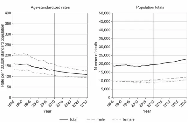
Observed and predicted age-standardized rates and counts of cancer mortality are shown in Figure 3. Predicted evolutions are similar to cancer incidence: The absolute number of cancer deaths will increase from 19,500 in 2009 to 20,900 in 2020 (+7%) and to 22,700 in 2030 (+16%). In contrast, age-standardized cancer mortality rates will decrease from 130 deaths per 100,000 standard population in 2009 to 117 in 2020 and then to 110 in 2030.
Figure 3: Observed (1985–2009) and predicted (2010–2030) mortality, all cancers
detection of cancers, or the reduction in tobacco smoking) dampens the aging-induced increase in cancer incidence and mortality.
Table 6: Comparison of model prediction with alternative constant rates scenario
Prediction outcome
Population totals
Predicted percentage change Observed in 2009 Predicted for 2030
Model (3) Constant rates
scenario Model (3)
Constant rates scenario
Incidence (newly diagnosed
cancers) 38,218 43,706 49,449 +14.4 +29.4 Mortality (cancer deaths) 19,547 22,707 26,909 +16.2 +37.7
3.2.2 Site-specific outcomes
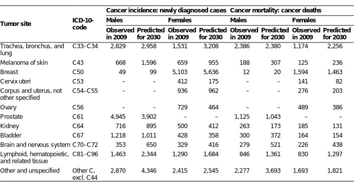
Table 7 presents the Austrian totals of newly diagnosed cancer cases and cancer deaths observed in 2009 and predicted for 2030, disaggregated by sex and tumor site. Values for 1983–2008 (observed) and for 2010–2029 (predicted) are available on request from the authors. Colon cancer incidence is predicted to increase among males but decrease among females. Colon cancer mortality is predicted to decline substantially among both sexes. Lung cancer diagnoses and deaths will remain rather constant among males but double among females. In 2030, more women than men will be newly diagnosed with lung cancer. Female breast cancer incidence will increase by about 10%, but deaths will decline by about 10% in 2009–2030. Some decline is also predicted for prostate cancer deaths. Stomach cancer incidence and mortality will decrease in the coming years. In contrast, newly diagnosed cases and deaths will rise for melanoma of skin, brain, and nervous system cancers, and cancers of lymphoid, hematopoietic, and related tissues.
Table 7: Predicted population totals of cancer incidence and cancer deaths by sex and tumor site
Tumor site ICD-10-code
Cancer incidence: newly diagnosed cases Cancer mortality: cancer deaths
Males Females Males Females
Observed in 2009 Predicted for 2030 Observed in 2009 Predicted for 2030 Observed in 2009 Predicted for 2030 Observed in 2009 Predicted for 2030
All cancers C00–C97, excl. C44
20,197 23,272 18,021 20,434 10,426 12,124 9,121 10,583
Head and neck C00–C10, C31–C32
864 820 282 409 355 370 128 269
Table 7: (Continued)
Tumor site ICD-10-code
Cancer incidence: newly diagnosed cases Cancer mortality: cancer deaths
Males Females Males Females
Observed in 2009 Predicted for 2030 Observed in 2009 Predicted for 2030 Observed in 2009 Predicted for 2030 Observed in 2009 Predicted for 2030
Trachea, bronchus, and lung
C33–C34 2,829 2,958 1,531 3,208 2,386 2,380 1,174 2,256
Melanoma of skin C43 668 1,596 659 955 188 307 125 236 Breast C50 49 99 5,103 5,636 12 20 1,594 1,463 Cervix uteri C53 – – 412 175 – – 141 82 Corpus and uterus, not
other specified
C54–C55 – – 936 962 – – 276 203
Ovary C56 – – 729 464 – – 489 386 Prostate C61 4,945 3,902 – – 1,125 1,043 – – Kidney C64 716 895 500 412 263 173 185 131 Bladder C67 1,218 1,011 428 358 300 372 164 154 Brain and nervous system C70–C72 353 650 329 416 279 521 226 438 Lymphoid, hematopoietic,
and related tissue
C81–C96 1,463 2,344 1,290 1,684 846 1,361 830 1,297
Other and unspecified Other C, excl. C44
2,870 4,346 2,415 2,545 2,277 3,693 1,693 1,821
Note: Predicted values are in general not integer-valued. In this table, predictions were rounded conventionally to next integers.
4. Discussion
4.1 Summary and comparison with international findings
The current paper aimed at predicting future cancer incidence and mortality rates for Austria in the midterm perspective up to 2030. Technically speaking, our prediction was a secondary population projection, i.e., we used a given population projection and applied forecasted cancer incidence and mortality rates to it. To our knowledge, ours is the first prediction of cancer cases that combines population projections with future rates obtained by quasi-likelihood regression models.
other authors (French, Catney, and Gavin 2006; Mistry et al. 2011; Rapiti et al. 2014). In the United States, the total cancer incidence is projected to increase by approximately 45% by 2030 (Smith et al. 2009).
We found decreasing trend parameters in the male and female cancer burden for most tumor sites. For lung cancer, however, we forecast a strong decrease in future incidence and mortality risk for males but a further increase for females. This difference is most likely a consequence of gender-specific behavioral changes because females are currently more likely to smoke, and males are less likely to do so compared to past decades (Statistik Austria 2015). To address this strong trend, also observable in other industrialized countries, Dyba and Hakulinen (2008) even sometimes exclude respiratory cancers from their cancer predictions. Respective predictions are also comparable for other countries. In Switzerland, age-standardized female lung cancer will increase by +48% by 2019, compared to +13% for males (Rapiti et al. 2014). On the contrary, little sex-specific variation in lung cancer trends up to 2030 is predicted for the United Kingdom (Mistry et al. 2011) and the United States (Smith et al. 2009). In a dynamic population health model using data from nine European countries, Lhachimi et al. (2016) estimated that smoking leads to 0.7 years and about 600,000 lives lost for males and 0.9 years and 700,000 lives lost for females. Although overall cancer incidence and death rates will decrease in Austria, the alarming lung cancer trends among women emphasize the need for evidence-based tobacco control interventions (Jemal et al. 2008).
Likewise, future head and neck cancer rates will increase in women but decrease in men. This finding is in line with a pooled analysis of international data conducted by Hashibe et al. (2009). As this tumor entity is also associated with smoking habits, this observation mirrors the trend seen in lung cancer. In addition to smoking and chewing tobacco products, alcohol use has been linked to head and neck cancer risk (Curado and Hashibe 2009; Roswall and Weiderpass 2015). One might speculate that with the social acceptance of tobacco and alcohol habits, women are adopting lifestyle habits that increase health risk previously accredited as “male” behavior (Wilsnack et al. 2018). Increasing both tobacco and alcohol prices could be feasible population-based measures to tackle unhealthy lifestyle habits (Turiano et al. 2015; Lhachimi et al. 2016).
We also estimated different parameter signs between males and females for the residual category “other and unspecified tumor site (other C, excl. C44).” However, this category is difficult to interpret due to its per se indistinctive nature. Thus, predictions concerning malignancies that fall into this category might benefit from specific research questions and assessments on a site-by-site basis, taking into account the site-specific trends and clinical features.
and given that Austria is a predominantly mountainous country, an ecological study found that melanoma incidence rates increased, whereas mortality rates decreased with altitude of place of living (Haluza, Simic, and Moshammer 2014). The observed diverging incidence and mortality trends might be explained by diagnosis at earlier tumor stages due to better screening adoption in these regions and vitamin D-driven slower tumor progression (Monshi et al. 2016). Also, upwelling radiation caused by, e.g., sunlight reflected by snow cover, could also explain higher melanoma incidence rates with altitude (Schrempf et al. 2016).
4.2 Uncertainty in our model predictions
Any prediction of future events naturally comes with uncertainty. As a general rule, the degree of uncertainty depends on the time horizon (the closer to the present, the more accurate) and on the plausibility and robustness of the underlying assumptions. Since our method combines two sources, a primary population projection and statistical model estimates, the overall uncertainty of our prediction has two components. In the following, we take the primary population projection as given and focus on uncertainty in the statistical model estimates.
4.2.1 Reliability
Figure 4: Prediction intervals for cancer incidence and cancer death counts
For the overall cancer incidence count in 2030, which we predict as 43,700, the confidence interval for the conditional expectation ranges from 43,500 to 43,900, and an approximate prediction interval for the actual outcome ranges from 43,200 to 44,200. For cancer death counts in 2030, predicted as 22,700, the confidence interval ranges from 22,500 to 22,900, and the approximate prediction interval from 22,300 to 23,100. So by any measure, uncertainty in our prediction caused by chance variation in the base period data is low and predictions are statistically reliable.
4.2.2 Validity
21 years is rather the upper limit of plausibility of assuming stable structural relationships.
Our model is essentially an exponential extrapolation of past trends into the future. We explicitly accounted for age structure and regional disparities and for known data artifacts such as changes in completeness of incidence case registration due to introduction of regional cancer registries during the base period. Developments such as change in risk behavior or medical and social progress are implicitly accounted for by the trend parameter. At least for prediction of all cancers combined, such superficially simple methods have often been found to be more useful than more sophisticated models that account for complex factors such as behavioral changes or population trends (Dyba and Hakulinen 2008; Statistik Austria 2015).
For some tumor sites in particular, estimated age group effects might be confounded by birth cohort effects, so age-specific forecasts might be somewhat biased. We abstained from accounting for birth cohorts in the statistical models because the data does not directly enable birth cohorts to be identified, and determining which cohort effects could be relevant for so many different models is not straightforward. Nevertheless, for forecasting specific cancer sites, e.g., female lung cancer, models that include cohort effects might be superior to our general approach.
The exponential term in the conditional mean specification is useful for predicting declining rates because forecasted rates never reach or fall below zero; however, the exponential term is less useful for rising rates because forecasted rates expand over time. However, since our prediction horizon is somewhat short (until 2030) and most time-trend parameters are indeed negative, this difference does not greatly affect the overall results. In contrast, French et al. (2006) apply an alternative method where falling rates are extrapolated exponentially, but rising rates linearly.
Forecasting separate trends by tumor site and sex has the advantage that different age profiles, etiologies, and trends are accounted for. This flexibility comes with the risk of inconsistencies between forecasted rates. This risk is exemplified by a male-female crossover of predicted pancreas cancer mortality rates and a singular decline in incident melanoma of the skin in Vienna compared to increases in all other Austrian regions. The convergence of male and female lung cancer rates, on the other hand, is not necessarily an inconsistency but is probably a consequence of the long-run convergence of smoking rates between men and women (Hackl and Waldhoer 2013).
5. Conclusion
In Austria, the absolute number of cancer cases increased continuously during the last decades. Our novel method combining population projections with quasi-likelihood models revealed that this trend will also continue in the near future due to the aging of the population, as cancer is primarily a disease of the elderly. On the contrary, age-standardized cancer incidence and mortality rates will decline substantially until 2030. Different trends are predicted by tumor site and for some tumor sites also by sex, region, or incidence vs. mortality.
6. Funding
This article is based on a study funded by the Austrian Federal Ministry of Health.
7. Acknowledgements
References
Ahmad, O.B., Boschi-Pinto, C., Lopez, A.D., Murray, C.J., Lozano, R., and Inoue, M. (2001). Age standardization of rates: A new WHO standard. Geneva: World Health Organization.
Anand, P., Kunnumakara, A.B., Sundaram, C., Harikumar, K.B., Tharakan, S.T., Lai, O.S., Sung, B., and Aggarwal, B.B. (2008). Cancer is a preventable disease that requires major lifestyle changes. Pharmaceutical Research 25(9): 2097–2116.
doi:10.1007/s11095-008-9661-9.
Bray, F. and Moller, B. (2006). Predicting the future burden of cancer.Nature Reviews Cancer6(1): 63–74.doi:10.1038/nrc1781.
Cameron, A.C. and Trivedi, P.K. (1998). Regression analysis of count data. Cambridge: Cambridge University Press.
CanReg5 (2016). Software [electronic resource]. La Jolla: SourceForge Media.
https://sourceforge.net/projects/canreg.
Curado, M.P. and Hashibe, M. (2009). Recent changes in the epidemiology of head and neck cancer. Current Opinions in Oncology 21(3): 194–200. doi:10.1097/CCO.
0b013e32832a68ca.
Doll, R. and Peto, R. (1981). The causes of cancer: Quantitative estimates of avoidable risks of cancer in the United States today. Journal of the National Cancer Institute 66(6): 1191–1308.doi:10.1093/jnci/66.6.1192.
Dyba, T. and Hakulinen, T. (2008). Do cancer predictions work?European Journal of Cancer 44(3): 448–453.doi:10.1016/j.ejca.2007.11.014.
Finkel, T., Serrano, M., and Blasco, M.A. (2007). The common biology of cancer and ageing.Nature 448(7155): 767–774.doi:10.1038/nature05985.
French, D., Catney, D., and Gavin, A.T. (2006). Modelling predictions of cancer deaths in Northern Ireland.Ulster Medical Journal 75(2): 120–125.
Hackl, M. and Waldhoer, T. (2013). Estimation of completeness of case ascertainment of Austrian cancer incidence data using the flow method. European Journal of Public Health 23(5): 889–893.doi:10.1093/eurpub/cks125.
Hanika, A. (2013). Zukünftige Bevölkerungsentwicklung Österreichs und der Bundesländer 2013 bis 2060 (2075). Statistische Nachrichten 68(11): 1005– 1024.
Hashibe, M., Brennan P., Chuang, S.-C., Boccia, S., Castellsague, X., Chen, C., Curado, M.P., Dal Maso, L., Daudt, A.W., and Fabianova, E. (2009). Interaction between tobacco and alcohol use and the risk of head and neck cancer: Pooled analysis in the International Head and Neck Cancer Epidemiology Consortium.
Cancer Epidemiology,Biomarkers and Prevention 18(2): 541–550.doi:10.1158/
1055-9965.EPI-08-0347.
Jemal, A., Thun, M.J., Ries, L.A., Howe, H.L., Weir, H.K., Center, M.M., Ward, E., Wu, X.C., Eheman, C., Anderson, R., Ajani, U.A., Kohler, B., and Edwards, B.K. (2008). Annual report to the nation on the status of cancer, 1975–2005, featuring trends in lung cancer, tobacco use, and tobacco control.Journal of the National Cancer Institute 100(23): 1672–1694.doi:10.1093/jnci/djn389.
Lhachimi, S.K., Nusselder, W.J., Smit, H.A., Baili, P., Bennett, K., Fernandez, E., Kulik, M.C., Lobstein, T., Pomerleau, J., Boshuizen, H.C., and Mackenbach, J.P. (2016). Potential health gains and health losses in eleven EU countries attainable through feasible prevalences of the life-style related risk factors alcohol, BMI, and smoking: A quantitative health impact assessment. BMC Public Health
16(734): 1–11.doi:10.1186/s12889-016-3299-z.
McCullagh, P. and Nelder, J.A. (1989). Generalized linear models. Second edition. Boca Raton: Chapman and Hall/CRC Press.
Mistry, M., Parkin, D.M., Ahmad, A.S., and Sasieni, P. (2011). Cancer incidence in the United Kingdom: Projections to the year 2030. British Journal of Cancer
105(11): 1795–1803.doi:10.1038/bjc.2011.430.
Moller, H., Fairley, L., Coupland, V., Okello, C., Green, M., Forman, D., Moller, B., and Bray, F. (2007). The future burden of cancer in England: Incidence and numbers of new patients in 2020. British Journal of Cancer 96(9): 1484–1488.
doi:10.1038/sj.bjc.6603746.
Monshi, B., Vujic, M., Kivaranovic, D., Sesti, A., Oberaigner, W., Vujic, I., Ortiz-Urda, S., Posch, C., Feichtinger, H., Hackl, M., and Rappersberger, K. (2016). The burden of malignant melanoma: Lessons to be learned from Austria. European Journal of Cancer 56: 45–53.doi:10.1016/j.ejca.2015.11.026.
Olsen, A.H., Parkin, D.M., and Sasieni, P. (2008). Cancer mortality in the United Kingdom: Projections to the year 2025.British Journal of Cancer 99(9): 1549– 1554.doi:10.1038/sj.bjc.6604710.
Preston, S.H., Heuveline, P., and Guillot, M. (2000). Demography: Measuring and modeling population processes. Malden: Wiley-Blackwell.
Rapiti, E., Guarnori, S., Pastoors, B., Miralbell, R., and Usel, M. (2014). Planning for the future: Cancer incidence projections in Switzerland up to 2019.BMC Public Health 14(102): 1–7.doi:10.1186/1471-2458-14-102.
Roswall, N. and Weiderpass, E. (2015). Alcohol as a risk factor for cancer: Existing evidence in a global perspective. Journal of Preventive Medicine and Public Health 48(1): 1–9.doi:10.3961/jpmph.14.052.
Schrempf, M., Haluza, D., Simic, S., Riechelmann, S., Graw, K., and Seckmeyer, G. (2016). Is multidirectional UV exposure responsible for increasing melanoma prevalence with altitude? A hypothesis based on calculations with a 3D-human exposure model. International Journal of Environmental Research and Public Health 13(961): 1–9.doi:10.3390/ijerph13100961.
Smith, B.D., Smith, G.L., Hurria, A., Hortobagyi, G.N., and Buchholz, T.A. (2009). Future of cancer incidence in the United States: Burdens upon an aging, changing nation.Journal of Clinical Oncology27(17): 2758–2765.doi:10.1200/
JCO.2008.20.8983.
Statistik Austria (2014). Nomenclature of Territorial Units for Statistics (NUTS) Austria [electronic resource]. Vienna: Statistik Austria. http://www.statistik.at/
web_en/classifications/regional_breakdown/nuts_units/index.html.
Statistik Austria (2015). Smoking habits of the Austrian population from 1972 to 2014 [electronic resource]. Vienna: Statistik Austria. http://statistik.at/web_de/ statistiken/menschen_und_gesellschaft/gesundheit/gesundheitsdeterminanten/rau
chen/025421.html.
Turiano, N.A., Chapman, B.P., Gruenewald, T.L., and Mroczek, D.K. (2015). Personality and the leading behavioral contributors of mortality. Health Psychology 34(1): 51–60.doi:10.1037/hea0000038.
Valls, J., Castella, G., Dyba, T., and Cleries, R. (2015). Selecting the minimum prediction base of historical data to perform 5-year predictions of the cancer burden: The GoF-optimal method. Cancer Epidemiology 39(3): 473–479.
Wilsnack, R.W., Wilsnack, S.C., Gmel, G., and Kantor, L.W. (2018). Gender differences in binge drinking.Alcohol Research 39(1): 57–76.
Appendix
Table A-1: Pooling of younger age groups in regression models, on the basis of incidences rates 2008–2010
Tumor site ICD-10 code Age-specific incidence rate in 2008–2010
#
Pooled age group 0–4 5–14 15–24 25–34 35–44 45–54
Head and neck C00–C10, C31–C32 0.3 0.0 0.4 0.8 4.0 19.7 0–34 Stomach C16 0.0 0.0 0.0 1.1 2.9 8.7 0–34 Colon, rectum, and anus C18–C21 0.0 0.1 0.7 2.3 9.2 30.8 0–24 Pancreas C25 0.0 0.0 0.1 0.3 2.0 9.8 0–34 Trachea, bronchus, and lung C33–C34 0.0 0.0 0.3 1.0 6.4 39.1 0–34 Melanoma of skin C43 0.1 0.3 3.6 8.5 13.6 16.8 0–14 Breast C50 0.0 0.0 0.6 7.4 36.9 80.5 0–24 Cervix uteri C53 0.0 0.0 0.3 3.4 6.0 6.6 0–24 Corpus and uterus, not other
specified C54–C55 0.0 0.0 0.0 0.5 2.0 8.8 0–34 Ovary C56 0.0 0.4 0.5 0.9 3.2 8.5 0–34 Prostate C61 0.0 0.0 0.0 0.1 1.9 27.7 0–34 Kidney C64 1.9 0.1 0.1 1.0 4.4 12.6 5–34 Bladder C67 0.0 0.0 0.3 0.6 2.4 8.9 0–34 Brain and nervous system C70–C72 3.5 2.5 2.0 3.3 4.3 8.1 – Lymphoid, hematopoietic, and
related tissue C81–C96 6.1 4.6 7.6 7.8 11.4 22.9 – Other and unspecified Other C, excl. C44 4.1 3.0 10.0 21.8 30.7 58.3 –
Note:#Age-specific incidence rates are newly diagnosed cancers per 100,000 person-years lived in the same age group.
Table A-2: Regression models where regionally different trend parameters were applied
Tumor site ICD-10 code Outcome (Groups of) NUTS-2 regions for which separate trend parameters were estimated# Colon, rectum, and anus C18–C21 Male incidence Styria, Tyrol, Vorarlberg – All other
Melanoma of skin C43 Male incidence Burgenland, Lower Austria – Vorarlberg. Vienna – All other
Female incidence Tyrol, Vienna – All other Male mortality Vienna – All other
Cervix uteri C53 Female incidence Carinthia, Upper Austria – All other Female mortality Burgenland, Vienna – Salzburg – All other Corpus and uterus not, other
specified
C54–C55 Female incidence Lower Austria – All other
Bladder C67 Male incidence Salzburg – All other Brain and nervous system C70–C72 Male incidence Styria – All other
Male mortality Vienna – All other Female mortality Vienna – All other Lymphoid, hematopoietic, and
related tissue
C81–C96 Male incidence Salzburg, Tyrol, Vorarlberg – All other Female incidence Salzburg, Vorarlberg – All other Other and unspecified Other C, excl. C44 Female incidence Carinthia, Upper Austria, Tyrol – All other
Table A-3: Estimated dispersion parameters
Tumor site ICD-10 code
Quasi-likelihood dispersion parameter Incidence Mortality
Males Females Males Females
Head and neck C00–C10, C31–C32 1.10 1.00 1.04 1.02 Stomach C16 1.05 1.03 1.03 1.05 Colon, rectum, and anus C18–C21 1.13 1.07 1.09 1.02 Pancreas C25 1.01 1.02 1.02 1.06 Trachea, bronchus, and lung C33–C34 1.19 1.12 1.17 1.08 Melanoma of skin C43 1.16 1.21 0.98 1.01 Breast C50 0.96 1.21 0.93 1.02 Cervix uteri C53 – 1.14 – 1.06 Corpus and uterus not, other specified C54–C55 – 1.05 – 1.07
Ovary C56 – 1.05 – 1.06