Web Appendix for “The (Un)importance of Geographical Mobility
in the Great Recession”
Siddharth Kothari, Itay Saporta-Eksten and Edison Yu
A
Methodology
In this section we provide a full derivation of our stock-flow equations followed by details on how we compound the counterfactual over time. We then formally describe the homeownership correction conducted in Section 7. Finally, we discuss the conditions which are required to get an upper bound for the effect of mobility on unemployment.
A.1
Stock-Flow Equation
The main equation that relates the unemployment stock of workers to the flows into and out of unemployment is given below1
Ut=Ut−1
−(UH,t−1∩MJt−1∩Et)
− UH,t−1∩MJt−1∩Et (A.1)
−(UR,t−1∩Et)
+Other Net in f lowt−1.
HereUt−1is the set of unemployed at timet−1;UH,t−1is the set of unemployed homeowners at timet−1;UR,t−1 is the set of unemployed renters at timet−1;MJt−1is the set of people who move for jobs between timet−1 andt (people whose labor market outcomes improve as a result of moving);MJt−1is the complement of the setMJt−1and includes all non-movers and people who move but their moves were not job related;Other Net in f lowt−1refers to all separations between employer and worker which lead to a transition of the worker from employment to unemployment betweent−1 andt, and to net inflows to unemployment from out of the labor force; andEt is the set of employed
people at timet.
Using shares and reorganizing, equation (A.1) becomes
Ut=Ut−1
−UH,t−1mU Ht−1jt−U H1 eU Ht−1−e¯U Ht−1
(A.2)
−UH,t−1e¯U Ht−1 −UR,t−1eU Rt−1 +Et−1δt−1
Where,mU Ht−1=UH,t−1∩Mt−1
UH,t−1 −moving rate among unemployed homeowners (Mt−1are all movers between t-1 and t);
jU H t−1=
UH,t−1∩MJt−1
UH,t−1∩Mt−1 −job-related moves as a share of all moves among unemployed homeowners;
1Because we only care about the level of unemployment and not about tracking specific individuals from unemployment to employment, it
would have been more accurate to replace each set in equation (A.1) by its cardinality (e.g., replaceUH,t−1∩MJt−1∩Etby|UH,t−1∩MJt−1∩Et|).
eU Ht−1=UH,t−1∩MJt−1∩Et
UH,t−1∩MJt−1 −share of unemployed homeowners who move for jobs and become employed by the next
period;
¯
eU Ht−1=UH,t−1∩MJt−1∩Et
UH,t−1∩MJt−1 −share of other unemployed homeowners who become employed by the next period
eU Rt−1=UR,t−1∩Et
UR,t−1 −share of unemployed renters who become employed by the next period; and
δt−1=Et−1
∩Ut
Et−1 −share of employed who become unemployed by the next period.
2
Collapsing the last three terms and naming itNt, equation (A.2) yields equation (1) in the paper. Ut=Ut−1−UH,t−1mU Ht−1jU Ht−1 eU Ht−1−e¯U Ht−1
+Nt (A.3)
where,Nt=−UH,t−1e¯U Ht−1−UR,t−1eU Rt−1+Et−1δt−1
A.2
Counterfactual Exercise
As noted in the paper, the counterfactual exercise is conducted by first recovering ˆNtand then boosting the mobility rate
of homeowners frommU Ht−1tomU Ht−1,C.3 For the first time period in which we run the counterfactual, the counterfactual unemployment level is given by
U1C=U0−UH,0mU H0 ,Cj
U H
0 eU H0 −e¯U H0
+Nˆ1. (A.4)
The subscript 0 represents the base period and 1 the first period of the counterfactual. For subsequent periods, the counterfactual unemployment rate is calculated by compounding the counterfactual from the previous period:
UtC=Ut−C1−UHC,t−1mU Ht−1,CjU Ht−1 eU Ht−1−e¯U Ht−1+Nˆt. (A.5)
Note that we also need to keep track of the counterfactual level of unemployed homeowners (UHC,t−1) because it appears on the right-hand side of equation (A.5). This is done using an equation that is similar to equation (A.3), but for unemployed homeowners. We can write the stock flow equation forUH,tas in the following:
UH,t=UH,t−1−UH,t−1mU Ht−1jU Ht−1 eU Ht−1−e¯U Ht−1
+NNt.
As with ˆNt, we can back out the residual termNNt by using data for the first two terms:
ˆ
NNt=UH,t−UH,t−1+UH,t−1mU Ht−1jU Ht−1 eU Ht−1−e¯U Ht−1
.
Then we can boost the probability of move to get the counterfactual unemployment level within the group of homeowners as
UHC,t=UHC,t−1−UHC,t−1m
U H,C t−1 j
U H
t−1 eU Ht−1−e¯U Ht−1
+NNˆ t, (A.6)
where for the base periodUHC,0=UH,0.
A.3
Homeownership Correction
In the CPS, we do not observe homeownership status prior to the move but only post-move. We therefore approximated the share of homeowners who moved,Ht−12∩Mt−12,by usingHt∩Mt−12. In this section we show how to construct a correction for the change in homeownership (conducted in Section 7 of the paper). This correction allows us to proxy
Ht−12∩Mt−12better at the cost of focusing on the population of 16- to 65-year-olds instead of only individuals in the labor force.2To ease notation, we assume that the labor force is fixed, andOther Net in f low
t−1therefore includes only transitions from employment to
unemployment.
3In some of the exercises we also take the counterfactual ofjU H
t . All the derivations are identical, and can be thought of as settingjU H0 =1 and
redefinigmU H
t−1as job-related mobility andm U H,C
We are interested in recovering the number of homeowners att−12 who moved betweent−12 andt. This number is given by
Ht−12∩Mt−12=Ht−12∩Mt−12∩Ht+Ht−12∩Mt−12∩Rt (A.7)
while the proxy measure which we have used for our baseline calculations is
Ht∩Mt−12=Ht−12∩Mt−12∩Ht+Rt−12∩Mt−12∩Ht
To get an accurate measure of (Ht−12∩Mt−12), we need to subtract from our baseline measure the number of renters who moved and became homeowners (Rt−12∩Mt−12∩Ht) and add the number of homeowners who moved
and became renters (Ht−12∩Mt−12∩Rt). Our correction is based on the observation that transitions from renting to
owning status and vice verse would most likely be accompanied by a move. Formally we assume
Ht−12∩Mt−12∩Rt ≈ Ht−12∩Rt (A.8)
Rt−12∩Mt−12∩Ht ≈ Rt−12∩Ht (A.9)
This allows us to relate our measures of interest (Rt−12∩Mt−12∩Ht andHt−12∩Mt−12∩Rt) to the change in the
numbers of homeowners and renters in the population given by
∆Ht = Ht−Ht−12=Rt−12∩Ht−Ht−12∩Rt+NHt
∆Rt = Rt−Rt−1=Ht−12∩Rt−Rt−12∩Ht+NRt
whereNHt andNRt are net new homeowners and net new renters (new in the sense of new to the population we
are looking at), respectively. We can use assumptions (A.8) and (A.9) (second equality in equation (A.10)) to write equation (A.7) as
Ht−12∩Mt−12 ≈ Ht∩Mt−12−∆Ht+NHt=Ht∩Mt−12+∆Rt−NRt (A.10)
WhileHt∩Mt−12,∆Ht and∆Rt are observed,NHt andNRt are not observed. To measureNHt, we would need
to know both how many people in the labor force today were not in the labor force in the last period and also their homeownership status. Since the CPS does not track the labor force status of individuals in the previous year, we cannot measureNHt when working with the labor force as our population. However, if we redefine our population as
all people in the age group of 16- to 65-year-olds, then we can measureNHt andNRt NHt = Ht∩[aget=16]−Ht−12∩[aget−12=65]
NRt = Rt∩[aget=16]−Rt−12∩[aget−12=65]
Given NHt andNRt, all the right-hand side variables in equation (A.10) are observed, implying that we can
calculateHt−12∩Mt−12.
A.4
Upper Bound - Propositions and Proof
In this section, we formalize under precisely what assumptions the results in the paper are an upper bound for the effect of mobility on unemployment. In particular, we show that there are two factors that make our counterfactual unemployment ratesmallerthan what the true counterfactual unemployment rate should be (i.e., we obtain anupper boundfor the effect of mobility on unemployment).
First, our counterfactual exercise ignores the effect of changing mobility on net flows which arenotdirectly related to job-related mobility (Nt). When we conduct the counterfactual exercise, we keepNtconstant and ignore the fact that higher mobility should also impact these net flows into unemployment. We start by showing under which assumptions, when compounding over more than one period, the measuredNt underestimates the flows into unemployment. This
Second, when conducting the counterfactual exercise, we use values for jU Ht−1,and eU Ht−1−e¯U Ht−1
that are higher than their values in the population. Moreover, for a given choice of counterfactual mobility, we try to boost the
differencemU Ht−1,C−mU Ht−1, which further exaggerates the effect of mobility on unemployment. We refer to this result asmeasurement upper boundand formalize it in Proposition 2.
A.4.1 Methodological Upper Bound
In the paper, we defined a job finding rate for all unemployed homeowners who do not move for job and called it ¯eU Ht−1. Here we further split this group into two groups - first, the group of unemployed homeowners who move for jobs only in the counterfactual i.e. who move for job in the counterfactual but do not do so in the observed world; second, the group who do not move for job both in the observed and in the counterfactual world. We define the job finding rate of these two groups as ¯eU Ht−1andeU Ht−1,NM respectively. The reason for this change is that our counterfactual exercise changes the composition of the group of unemployed homeowners who do not move for jobs. In the counterfactual world, the size of the group shrinks as some of the unemployed in this group move for jobs and are assigned the higher job-finding rateeU H
t−1. By defining two job finding rates, we clarify how this composition shift impacts our counterfactual exercise.
Proposition1: Define UtCI to be the true counterfactual that takes into account the effect of change in mobility rate on Nt. The following conditions aresufficientfor UtC (as defined in equation (A.5)) to be a lower bound (upper bound for the effect of mobility), i.e. UtC6UtCI,∀t:
(C.1)δt, jU Ht , and all finding rates(eU H, e¯tU H,eU Ht−1,NMand eU Rt )are not changing in the counterfactual∀t. (C.2) mU Ht−1,Cjt−U H1eU Ht−1−eU Ht−1,NM+eU Ht−1,NM+δt−1≤1
Proof:We start by showing thatU1C=U1CI holds. Equation (A.2) becomes
Ut=Ut−1
−UH,t−1mU Ht−1jt−U H1 eU Ht−1−e¯U Ht−1
−UH,t−1mU Ht−1,Cj
U H t−1e¯U Ht−1 −UH,t−1
h
1−mU Ht−1,CjU Ht−1ieU Ht−1,NM
−UR,t−1eU Rt−1 +Et−1δt−1
where for a givenmU Ht−1,C, the third line refers to the group of individuals who move for job in the counterfactual. Define
ˆ
Nt=Ut−Ut−1+UH,t−1mU Ht−1jU Ht−1 eU Ht−1−e¯U Ht−1
and the counterfactual becomes
UtC=Ut−C1−UHC,t−1m
U H,C t−1 j
U H
t−1 eU Ht−1−e¯U Ht−1
+Ntˆ
which for the first period implies
U1C=U1−UH,0
mU H0 ,C−mU H0
jU H0 eU H0 −e¯U H0 (A.11)
The true counterfactual for period 1,UtCI is given by
U1CI=U0
−UH,0mU H0 ,Cj
U H
0 eU H0 −UH,0
h
1−mU H0 ,CjU H0 ieU H0 ,NM
Adding and subtractingU1from this equation we get
U1CI=U1−UH,0
mU H0 ,C−mU H0 jU H0 eU H0 −e¯U H0
=U1C (A.12)
We show now how to obtain an upper bound with compounding. Define the differences of observed unemployment and (true) counterfactual unemployment as the following:
∆UtC ≡ Ut−UtC
∆UHC,t ≡ UH,t−UHC,t
∆UtCI ≡ Ut−UtCI
∆UHCI,t ≡ UH,t−UHCI,t
Using this notations, we can express these differences as a set of first order linear difference equations
∆UtC = ∆Ut−C1+UH,t−1
mU Ht−1,C−mU Ht−1jt−U H1 eU Ht−1−e¯U Ht−1 (A.13) −∆UHC,t−1m
U H,C t−1 j
U H
t−1 eU Ht−1−e¯U Ht−1
∆UHC,t = ∆Ut−C1+UH,t−1
mU Ht−1,C−mU Ht−1
jU Ht−1 eU Ht−1−e¯U Ht−1
(A.14)
−∆UHC,t−1m
U H,C
t−1 jU Ht−1 eU Ht−1−e¯U Ht−1
∆UtCI = ∆Ut−CI1+UH,t−1
mU Ht−1,C−mU Ht−1jU Ht−1 eU Ht−1−e¯U Ht−1 −∆UHCI,t−1m
U H,C t−1 j
U H
t−1 eU Ht−1−e¯U Ht−1
−∆UHCI,t−1m
U H,C t−1 j
U H
t−1e¯U Ht−1 (A.15) −∆UHCI,t−1
h
1−mU Ht−1,CjU Ht−1 i
eU Ht−1,NM−∆UHCI,t−1δt−1
∆UHCI,t = ∆UHCI,t−1+UH,t−1
mU Ht−1,C−mU Ht−1
jU Ht−1 eU Ht−1−e¯U Ht−1
−∆UHCI,t−1m
U H,C t−1 j
U H
t−1 eU Ht−1−e¯U Ht−1
−∆UHCI,t−1m
U H,C t−1 j
U H
t−1e¯U Ht−1 (A.16) −∆UHCI,t−1
h
1−mU Ht−1,CjU Ht−1iet−U H1,NM−∆UHCI,t−1δt−1
where, in the base period ∆U0C=∆UHC,0=∆U0CI =∆UHCI,0=0. It is easy to recognize that ∆UtC=∆UHC,t, and ∆UtCI=∆UHCI,t,∀t>0. Hence, if the ultimate goal is to signUtCI−UtC=∆UtC−∆UtCI, it is sufficient to examine the
sign of∆UHC,t−∆UHCI,t.
We prove the proposition by induction. We know that∆UHC,1−∆UHCI,1=0.
Now assume that∆UHC,t−1−∆UHCI,t−1>0 and∆UHCI,t−1≥0. If we can prove that∆UHC,t−∆UHCI,t≥0 and∆UHCI,t≥0, then we are done.
Taking the difference of equation (A.14) and (A.16), and rearranging gives
∆UtC−∆UtCI = ∆UHC,t−1−∆UHCI,t−1
h
1−mU Ht−1,CjU Ht−1 eU Ht−1−e¯U Ht−1
i
+ ∆UHCI,t−1 h
mU Ht−1,CjU Ht−1e¯U Ht−1+
1−mU Ht−1,CjU Ht−1
eU Ht−1,NM+δt−1 i
The induction assumptions were that∆UHC,t−1−∆UHCI,t−1≥0 and∆UHCI,t−1≥0. Therefore, all terms in the above equation are greater than zero. Therefore,∆UHC,t−∆UHCI,t≥0
To complete the proof we need to show that∆UHCI,t≥0. Rearranging equation (A.16) we get
∆UHCI,t = ∆UHCI,t−1 h
1−mU Ht−1,CjU Ht−1eU Ht−1−eU Ht−1,NM−eU Ht−1,NM−δt−1 i
+UH,t−1
Notice that the above equation is simply an AR(1) in ∆UHCI,t but with coefficients which are time varying. In
particular,
∆UHCI,t=bt−1∆UHCI,t−1+at−1 wherebt−1=1−mt−U H1,CjU Ht−1
eU Ht−1−eU Ht−1,NM
−eU Ht−1,NM−δt−1andat=UH,t−1
mU Ht−1,C−mU Ht−1
jU Ht−1 eU Ht−1−e¯U Ht−1≥ 0.
Under the induction assumption that∆UHCI,t−1≥0, a sufficient condition for∆UHCI,t≥0 is thatbt≥0 i.e. mU Ht−1,CjU Ht−1eU Ht−1−et−U H1,NM+eU Ht−1,NM+δt−1≤1.
We address assumption C.1 in footnote 10 in the paper. Note that this assumption gives sufficient, but not necessary conditions for ˆNt to overstate the ideal counterfactual residual flow into unemployment. Note that assumption (C.2) is
a technical assumption related to compounding. In particular, it is required to rule out the pathological case in which increased mobility actually leads to higher unemployment (i.e.,UtCI>Ut).
A.4.2 Measurement Upper Bound
We turn now to show that when we measuremU Ht ,C−mU Ht ,jU Ht and eU Ht −e¯U Ht with an upward bias, we amplify the effect of mobility on unemployment even further. Proposition 2 shows this for a single period counterfactual. We find it useful to state the proposition for a single period because the bias for this case is very easy to calculate. The proposition and proof extending this result to multiple periods are available upon request.
Let ˜mU H
t , ˜jU Ht ,e˜¯U Ht and ˜eU Ht be the measured values ofmU Ht , jU Ht , e¯U Ht andeU Ht and ˜m U H,C
t be the counterfactual
mobility rate used. ˆN1andU1Care now given by ˆ
N1=U1−U0+UH,0m˜U H0 j˜U H0 e˜U H0 −e˜¯U H0
U1C=U0C−UH,0m˜0U H,Cj˜U H0 e˜U H0 −e˜¯U H0
+Nˆ1 (A.17)
Proposition 2:Let time0be the base period and U1CI be the true counterfactual that takes into account the effect of change in mobility rate on N1. The following conditions aresufficientfor U1C(as defined in equation (A.17)) to be
a lower bound (upper bound for the effect of mobility), i.e. U1C6U1CI: (C.1) holds for t=0
(C.3)m˜U H0 ,C−m˜U H0 ≥mU H0 ,C−mU H0 , ˜jU H0 ≥jU H0 and ˜eU H0 −e˜¯U H0 ≥eU H0 −e¯U H0
Proof:Equation (A.12) is unchanged, but equation (A.11) should be now written as
U1C = U1−UH,0j˜U H0 e˜U H0 −e˜¯U Ht
(m˜U H0 ,C−m˜U H0 ) (A.18) Taking the difference of equations (A.18) and (A.11) we get
U1CI−U1C = UH,0(m˜U H0 ,C−m˜
U H
0 )j˜U H0 e˜U H0 −e˜¯U Ht
−UH,0
mU H0 ,C−mU H0 jU H0 eU H0 −e¯U H0 = UH,0
h
(m˜U H0 ,C−m˜U H0 )j˜U H
0 e˜U H0 −e˜¯U Ht
−mU H0 ,C−mU H0 jU H0 eU H0 −e¯U H0 i≥0
where the last inequality is using assumption(C.3).
The intuition for assumption (C.3) is as follows: ˜mU H0 ,C−m˜U H
0 ≥m
U H,C
0 −mU H0 and ˜jU H0 ≥jU H0 ensure that the size of the group of interest (movers for jobs) is overestimated. ˜eU H
0 −e˜¯U H0 ≥eU H0 −e¯U H0 further ensures that the mobility-related flows out of unemployment for any given size of the group is also overestimated.
rate of 1 for movers for jobs and of 0 for all other homeowners. If all other parameters are set to their population values, our counterfactual exercise in the first period overstates the effect of mobility by
U1−U1C
U1−U1CI
= 1
eU H0 −e¯U H0
Keeping the finding rate for movers for jobs (eU H0 ) at the upper bound of 1, and assigning 0.23 (the average monthly hazard rate during the Great Recession calculated using the method in Shimer (2005)) to the finding rate for all homeowner ( ¯eU H0 ), our counterfactual exercise overstates the effect of mobility on unemployment by about 30%.
Note that when choosing mobility rates, we boost both ˜mU H0 ,C andm˜U H0 proportionally (using the PSID to get to unemployed mobility from total mobility). This is an effort to make the difference ˜mU H0 ,C−m˜U H0 also larger than the true population value.
B
Data Appendix
We use data from three sources:
1. March CPS - We use the Annual Social and Economic Supplement (ASEC) to the Current Population Survey (CPS) as the main source of data for mobility and reason for move. The data from 1980 to 2011 comes from IPUMS-CPS.4 For 2005 to 2012, we also use the NBER March CPS files to construct a panel of matched individuals over time and between monthly and March files, as matching is not possible using the IPUMS data.5
2. Monthly CPS Data - We use the monthly CPS public use files to generate monthly estimates of unemployment for homeowners and renters. We also use the monthly files when constructing our measure of mobility based on non-matches in the CPS. The source of the data is NBER and the US Census Bureau.6
3. Panel Study of Income Dynamics (PSID) - We use the PSID to calculate (mU Ht
mtH
) and (mU Rt
mRt
), as explained below.7
We go through our key measures in details below.
B.1
Key Mobility Measures
We measure total as well as inter-county mobility rates by using the March CPS. Since our exercise is focused on 2006 and onwards, our inter-county mobility rates are not exposed to the criticism made by Kaplan and Schulhofer-Wohl (2012a) regarding changes in the imputation procedures of mobility. We therefore include imputed values in our analysis. The advantage of that is that it allows us to calculate true mobility rates by dividing the number of moves betweentandt+1 by the relevant population at timet, and not att+1 (this could be a problem if dropping imputed values, and the total weight of imputed observations is changing over time).8 One exception is the data presented in Section 2 (and the accompanying Table A.1). As this section reviews long term trends, we do exclude imputed values from our analysis, and dividettot+1 moves byt+1 population.
For our counterfactual exercise, we want to correct our measured mobility rates for the possibility that unemployed homeowners move more than all homeowners. We used the Panel Study of Income Dynamics (PSID) to construct the
ratio mU Ht
mHt
, wheremHt is mobility rate for all homeowners. Table A.2 provides the annual values of the ratio mU Ht
mHt
for homeowners and renters in columns 1 and 2 respectively. Note that the PSID becomes bi-annual after 1997. As the table shows, the ratio fluctuates a lot from year to year. Keeping this in mind, we do not take the value of this ratio from
4See http://cps.ipums.org/cps/ and King et al. (2010) for more details.
5See the NBER page with CPS March data: http://www.nber.org/data/current-population-survey-data.html. This is only used for footnote 10 of
this web appendix.
6See http://www.nber.org/data/cps_basic.html and http://dataferrett.census.gov/ respectively for more details. 7http://psidonline.isr.umich.edu/
8The projection used in Table 1, column 2, Panel B uses inter-county data from 2001 for the projection, therefore potentially sensitive to the
1 year but rather average over the 5 highest years. Despite these caveat, it is interesting to note that while the highest value for the ratio in the last twenty years is 1.97, the ratio was consistently around 2 during the twin recessions of the early 1980’s and during the subsequent recovery. Also, the ratio of mobility for unemployed renters to total mobility of renters is generally a lot smaller, with a highest value of 1.25 in 1999.
We use self reported reason for move to distinguish job related moves from other moves. We try to take the broadest measure for mobility for job-related reasons, classifying the following answers to the why moved question in the CPS as moving for a job: “new job or job transfer”, “to look for work or job lost”, “for easier commute”, “other job-related reason”. The measured shares of movers for jobs among movers is presented in Table A.3. The first column shows the ratio for homeowners, and the second column for renters.
Finally, Table A.4 provides the distribution of movers over reason for move for the year 2006 from the CPS. Columns 1 and 2 give the distribution for homeowners and renters for all movers. Columns 3 and 4 give the distribution for homeowners and renters for inter-county movers only. The first four rows represent the categories that we consider to be job-related moves. Job-related moves were only about 16% of all moves and about 30% of inter-county moves for homeowners.
B.2
Renters Reweighting
We construct a measure of renter mobility which accounts for the fact the renters are different than homeowners on observable characteristics. To do that, we first run probit regressions by year (weighted by CPS weights) of mobility indicator on a set of demographic characteristic, focusing only on the renters sample. We then use our estimates to predict the probability of move for homeowners, and aggregate up using the homeowners weights.
In the choice of demographic characteristic to include in our probit regressions, we follow loosely the set of demographic characteristics surveyed by Kaplan and Schulhofer-Wohl (2012b) in the context of the long term trend in mobility, and include age categories, education categories (and and interaction of age and education), marital status, number of labor force participants in the households, income percentiles and number of family members.
B.3
Mobility Based on CPS Non-match Rate
In section 7, we use a measure of mobility based on the non-match rate in the CPS. The CPS is an address based panel. The non-match rate of the CPS from month to month is therefore informative about mobility.
Each sample housing unit in the CPS is interviewed 8 times. When a housing unit is first picked in the CPS sample, it is interviewed for 4 consecutive months. This is followed by an 8 month break and then another 4 months of interviews. Therefore at any one point, there are housing units which might have had between 1 to 8 interviews. If the number of interviews that a housing unit has given so far is between 1 to 3, or between 5 to 7, then the housing unit should appear again in the next month of the sample. If it does not (or if it does but the age, sex, or race of the household members has changed, see for example Madrian and Lefgren (1999)), then we can classify the household or the individual staying in the housing unit as someone who has moved. This non-match based mobility measure has the advantage that it is monthly, and that homeownership and unemployment status are observed pre-move. The disadvantage is that other than mobility, sources of non-matches include non-response, mortality and recording errors.
C
Standard Errors Calculation
We provide details on how we compute the standard errors reported in Tables 1 and 2 of the paper. We compute the
standard error ofU2012m03−U2012C m03
LF2012,m03 ,using an iterative delta method.
First define
A0= [UH,2007m03...UH,2012m03,LF2012,m03,m2008∗j2008...m2012∗j2012,mC2008∗jC2012...mC2012∗jC2012]
0
force in March 2012,m2008∗j2008...m2012∗j2012are the shares of job-related moves among unemployed homeown-ers measured from the March CPS from 2008 to 2012, andmC2008∗ jC2012...mC2012∗jC2012are the counterfactual shares of job-related moves among unemployed homeowners.9 Given the covariance matrix ofA0, we can apply the delta method to find the covariance matrix of
A1= [UHC,2007m04,UH,2007m04...UH,2012m03,LF2012,m03,m2008∗j2008...m2012∗j2012,mC2008∗jC2012...mC2012∗jC2012]
0
asA1is just a function ofA0. Note thatUH,2007m03has been replaced byUHC,2007m04inA1. Similarly, the covariance matrix ofA1can be used to compute the covariance matrix of
A1= [UHC,2007m05,UH,2007m05...UH,2012m03,LF2012,m03,m2008∗j2008...m2012∗j2012,mC2008∗jC2012...mC2012∗jC2012]
0
This iterative process can be repeated till we find the covariance matrix of
A60= [UHC,2012m03,UH,2012m03,LF2012,m03,m2008∗j2008...m2012∗j2012,mC2008∗jC2012...mC2012∗jC2012]
0
and then as a final step apply the delta method again to estimate the variance ofUH,2012m03−U
C H,2012m03
LF2012,m03 .
In order to implement this procedure we need to first estimate the covariance matrix ofA0. We do this in two steps. First we estimate the covariance matrix ofAU= [UH,2007m03...UH,2012m03,LF2012,m03]0. We do this by running a stacked regression of the form
uit=αt+εit (C.1)
whereiindexes individuals,uit is a dummy which takes value 1 if individualiis an unemployed homeowner at time t. Using CPS weights,uit is regressed on a set of dummies, where each dummy takes value 1 for one month only.
The coefficients on these dummies are the estimates forαt, the share of unemployed homeowners at timet. To also
compute the covariance ofLF2012,m03, we add an additional set of observations for all individuals in March 2012 on the left hand side which take value 1 for people in the labor force. We add an additional dummy on the right hand side which takes value one for only these additional observations.
The CPS sample design requires clustering at the primary sampling units level (PSU) which is the size of a county or an MSA. In addition, when using estimates from consecutive cross-sections, one needs to take into account the rotating panel structure of the CPS. Unfortunately, the PSU is not part of the public use micro data. We therefore compute the variance ofαt by applying two way clustering. We allow for correlation within households over time by
clustering at the household level. We also cluster at the MSA level (we assign all individuals in a state whose MSA is not identified into a single group by state), which is a more conservative than the actual PSU stratification of the CPS. We then apply the CPS weights to recover the covariance matrix of unemployment levels.
In addition to the covariance matrix ofAU, we need the covariance matrix ofAM= [m2008∗j2008...m2012∗j2012,mC2008∗
jC2012...mC2012∗jC2012]0. For specifications that use renters mobility in the counterfactual, we first compute the covariance matrix of[m2008∗j2008...m2012∗j2012]by assuming that it is diagonal and estimate the diagonal elements by using the replicate weights provided with the March CPS.mC2008∗jC2012...mC2012∗jC2012is a function of job-related mobility of unemployed homeowners in 2007 mH2007∗jH2007, and job-related mobility rates for renters from 2007 to 2012
mR2007∗jR2007, ...,m2007R ∗j2012R . We estimate the covariance matrix ofmH2007∗jH2007,mR2007∗j2007R , ...,mR2007∗jR2012
by assuming that it is diagonal and computing the diagonal elements by using replicate weights and then apply the delta method to get the covariance matrix of
mC2008∗jC2012...mC
2012∗jC2012
. All the specifications which do not use renters as counterfactual, use only a single number mCt for all years, and also use jCt = jt. We account for
that in two ways: First, we only assume that the covariance matrix for [m2008...m2012,mCt]0 is diagonal and
cal-culate it with replicate weights. We then assign cov mCt,mCs=var mCt for all years when constructing the co-variance matrix for[m2008...m2012,mC2008...mC2012]0. Second, we use replicate weights to calculate a diagonal
covari-9Note that we include only the number of unemployed homeowners in the vectorA
0and not the total number of unemployed in each month. This
is becauseUH,2012m03−U
C H,2012m03
LF2012,m03 =
U2012m03−U2012C m03
LF2012,m03 in our exercise. Therefore, finding the variance of
UH,2012m03−UHC,2012m03
LF2012,m03 is equivalent to finding
the variance ofU2012m03−U2012C m03
LF2012,m03 and the former is a function of number of unemployed homeowners only and not of the total number of unemployed
ance matrix for[j2008...j2012]0. We then apply delta method to calculate the (non-diagonal) covariance matrix for [m2008∗j2008...m2012∗j2012,m2008C ∗j2012...mC2012∗j2012]0.10
References
Kaplan, Greg, and Sam Schulhofer-Wohl.2012a. “Interstate Migration Has Fallen Less Than You Think: Conse-quences of Hot Deck Imputation in the Current Population Survey.”Demography, 49(3): 1061–1074.
Kaplan, Greg, and Sam Schulhofer-Wohl. 2012b. “Understanding the long-run decline in interstate migration.” Federal Reserve Bank of Minneapolis Working Papers 697.
King, Miriam, Steven Ruggles, J. Trent Alexander, Sarah Flood, Katie Genadek, Matthew B. Schroeder, Bran-don Trampe, and Rebecca Vick. 2010. “Integrated Public Use Microdata Series, Current Population Survey: Version 3.0. [Machine-readable database].” Minneapolis: University of Minnesota.
Madrian, Brigitte C., and Lars John Lefgren. 1999. “A Note on Longitudinally Matching Current Population Survey (CPS) Respondents.” National Bureau of Economic Research, Inc NBER Technical Working Papers 0247.
Shimer, Robert.2005. “The Cyclical Behavior of Equilibrium Unemployment and Vacancies.”American Economic Review, 95(1): 25–49.
10We always impose the assumption of diagonal covariance matrix for the values which are calculated using replicate weights. This is not
necessarily true in the data, however in many specification, there is no other way to calculate the full covariance matrix. We check to see what the impact of non-zero covariances is on our standard error estimates for the baseline specification. For our baseline specification (Table 1, panel A, column 1), we computed the entire covariance matrix forA0, by including dummies for mobility (mt), counterfactual mobility (mCt) and job related
mobility (jt) in the regression in equation (C.1) again allowing for two way clustering. We then compared the standard errors from this covariance
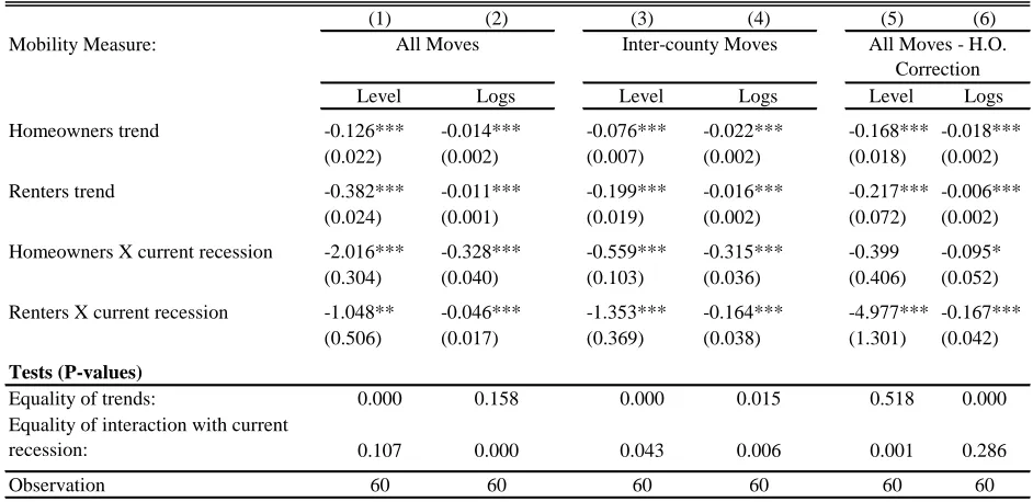
Table A.1: Homeowner and Renter Mobility over Time
(1) (2) (3) (4) (5) (6)
Mobility Measure:
Level Logs Level Logs Level Logs
Homeowners trend -0.126*** -0.014*** -0.076*** -0.022*** -0.168*** -0.018***
(0.022) (0.002) (0.007) (0.002) (0.018) (0.002)
Renters trend -0.382*** -0.011*** -0.199*** -0.016*** -0.217*** -0.006***
(0.024) (0.001) (0.019) (0.002) (0.072) (0.002)
Homeowners X current recession -2.016*** -0.328*** -0.559*** -0.315*** -0.399 -0.095*
(0.304) (0.040) (0.103) (0.036) (0.406) (0.052)
Renters X current recession -1.048** -0.046*** -1.353*** -0.164*** -4.977*** -0.167***
(0.506) (0.017) (0.369) (0.038) (1.301) (0.042)
Tests (P-values)
Equality of trends: 0.000 0.158 0.000 0.015 0.518 0.000
Equality of interaction with current
recession: 0.107 0.000 0.043 0.006 0.001 0.286
Observation 60 60 60 60 60 60
Notes: The table reports the results from the regression of annual mobility rates on dummies for homeowners and renters (not reported) and the interactions of a time trend and a current recession dummy with homeowner and renter dummies, with no constant. Current recession dummy equals 1 starting 2007. Mobility rates are calculated as the share of homeowners and renters in the labor force at t+1 who move between t and t+1 based on the March CPS for three mobility measures: All Moves (Columns 1, 2); Only inter-county moves (Columns 3, 4); All Moves, correcting for post-move recorded homeownership (Columns 5, 6). The time period is 1980 to 2011, where 1984 and 1994 are excluded, since mobility is not reported in CPS for these years. Observations with imputed migration data were removed for columns 1-4. Robust standard errors are reported. *** p<0.01, ** p<0.05, * p<0.1
All Moves Inter-county Moves All Moves - H.O.
TABLEA.2: MOBILITY OFUNEMPLOYED BYMOBILITY FORALL- PSID
(1) Mobility of Unemployed by Mobility of All -
Homeowners (%)
(2) Mobility of Unemployed by Mobility of All -
Renters (%)
1981 2.20 1.09
1982 2.09 1.07
1983 2.06 1.01
1984 1.70 1.09
1985 1.66 1.05
1986 2.00 0.86
1987 0.89 1.03
1988 2.59 1.01
1989 1.49 1.20
1990 1.15 1.04
1991 1.09 1.17
1992 1.43 1.18
1993 1.97 1.17
1994 1.30 0.97
1995 0.82 0.99
1996 0.87 0.80
1997 0.61 0.80
1999 1.69 1.25
2001 1.17 1.16
2003 1.07 0.86
2005 1.00 0.76
2007 1.18 0.98
2009 0.86 1.10
TABLEA.3: MOBILITY FORJOB ASSHARE OFMOVERS
(1) Move for job -
Homeowners (%)
(2) Moving for Job -
Renters (%)
2006 15.40 22.47
2007 17.65 24.76
2008 16.74 25.45
2009 14.73 21.76
2010 14.47 20.33
2011 16.35 22.42
2012 16.30 23.99
Notes: From the March CPS supplement using CPS weights. Columns (1) and (2) show the share of all movers who move for job related reasons among homeowners and renters respectively. Timing for all columns is from t-1 to t
TABLEA.4: DISTRIBUTION OFMOVERSOVERREASON FORMOVE
(1) Reason for Move, All
Moves - Homeowners
(%)
(2) Reason for Move, All
Moves - Renters
(%)
(3) Reason for Move,
Inter-county - Homeowners
(%)
(4) Reason for Move,
Inter-county - Renters
(%)
New job or job transfer 7.13 11.19 17.32 24.93
To look for work or lost job 2.03 1.93 4.42 4.21
For easier commute 3.60 4.99 5.08 6.19
Other job-related reason 2.64 4.36 3.44 6.99
Change in marital status 7.49 6.03 7.10 5.46
To establish own household 6.43 11.41 5.28 6.12
Other family reason 10.28 11.26 13.93 13.36
Retired 0.27 0.18 0.67 0.51
Wanted to own home, not rent 24.09 1.24 13.91 0.81
Wanted new or better housing 16.49 18.45 8.02 6.67
Wanted better neighborhood 4.56 3.92 4.95 2.52
For cheaper housing 3.59 7.39 3.78 3.83
Other housing reason 5.55 10.24 3.91 4.61
Attend/leave college 1.23 3.51 2.27 6.48
Change of climate 0.32 0.54 0.79 1.14
Health reasons 0.59 0.68 0.78 1.20
Other reasons 2.67 1.36 2.90 2.33
Natural disaster 1.04 1.31 1.43 2.64