Impurities in a Bose-Einstein condensate using quantum Monte-Carlo methods: ground-state properties.

(1)

(2)

(3)

Acknowledgements

ENGLISH VERSION (To the BEC crew)

It has been a long road until arrive here, sometimes a snaky road. But out of doubt getting this point it wouldn’t have been possible without many people who push me forwards in the moments of frustration and dismay.

From the bottom of my heart I am tremendously grateful with Stefano Giorgini, no only because his role as advisor, but for his invaluable guidance, patience and love for physics. I learnt from him an invaluable lesson that quality work always comes in a price: time, patience and discipline. Along the PhD many question popping into my mind and he was there to show me a light. I always will thanks Stefano, not only for his encourage but also for pointing out my weakness as well as to highlight in every meeting we had "...you must learn..."

I want to extend my thanks to Professor Sandro Stringari who allowed me to be part of this family and permit me to learn from outstanding people when I participated in conferences and workshops. Every single conference was an opportunity to inspire myself to continue in this beautiful path of research. Also being inspired every single day by the brilliant team at Trento Lev Pitaevskii, Franco Dalfovo, Iacopo Carusotto, Chiara Menotti, Alessio Recati, Gabriele Ferrari and Giacomo Lamporesi.

Heartfelt thanks to all the crew of the BEC group. In particular to David Papoular and Marta Abad for their help in many concerns and to my friends Grazia Salerno, Giovanni Martone and Yan-Hua Hou. As well as Giulia De Rosi, José Lebreuilly Nicola Bartolo, Simone Donadello, Stefano Finazzi, Marco Larcher, Pierre-Elie Larre, Natalia Matveeva, Tomoki Ozawa, Hannah Price, Riccardo Rota, Alberto Sartori, Robin Scott, Simone Serafini, Marek Tylutki, Zeng-Qiang Yu, Peng Zou, Li yun, and Onur Umucalilar.

My thanks are extended to the wonderful secretaries, Flavia Zanon, Micaela Paoli, Rachele Zanchetta and the technician Giuseppe Fronter whom provided the elements to be my stay more pleasant.

(4)

this thesis. On the other hand, I would like to thank to Professor Rudolf Grimm and Marko Cetina who gave me the opportunity for discussing about the experimental issues of the polaron problem. It was really tough but amazing, to learn and get involved in the discussions.

ITALIAN VERSION (To my girlfriend and the open space people)

Vorrei ringraziare la mia ragazza roberta, é stata al mio fianco anche nei momenti di sgomento e tristezza (...) Ha sempre trovato il modo di incoraggiarmi. Senza dubbio ho trovato un tesoro prezioso sulla mia strada del dottorato. Questa tesi é dedicata alla mia famiglia e alla mia Roby.

Grazie a Giovanna e Mary perché hanno fatto dell’ open space un posto più piacevole. Ringrazio la sua amicizia

SPANISH VERSION (To my family and my friends) Las más grandes gracias a mis padres, que a pesar de la distancia han estado siempre conmigo en este proceso desde que era un niño. Ellos son los únicos que han estado al tanto de mis pasos desde mi primera vez, cuando hice mi primaria en escuala muy vieja donde nos sentabamos en el suelo debido a la precaria situación económica hasta el punto el que he sido muy el privilegio y he aprendido un montón de cosas. Esta thesis es dedicada a ellos y mi adorada novia.

(5)

Abstract

In this thesis we investigate the properties of impurities immersed in a dilute Bose gas at zero temperature using quantum Monte-Carlo methods. The interactions between bosons are modeled by a hard sphere potential with scattering length a, whereas the interactions between

the impurity and the bosons are modeled by a short-range, square-well potential where both the sign and the strength of the scattering length b can be varied by adjusting the well depth. We

calculate the binding energy, the effective mass and the pair correlation functions of a impurity along the attractive and the repulsive polaron branch. In particular, at the unitary limit of the impurity-bosons interaction, we find that the binding energy is much larger than the chemical potential of the bath signaling that many bosons dress the impurity thereby lowering its energy and increasing its effective mass. We characterize this state by calculating the bosons-boson pair correlation function and by investigating the dependence of the binding energy on the gas parameter of the bosonic bath. We also investigate the ground-state properties of M impurities in a Bose gas atT=0. In particular, the energy and the phase diagram by using both quantum

(10)

(11)

List of Figures

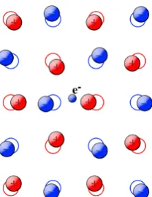
1.1 The ions placed on the lattice fell the attraction by the electron, therefore there is a distortion of the lattice. This electron and this distortion can be described by a quasiparticle with different mass and energy respect the naked electron and this quasiparticle is called polaron. . . 14

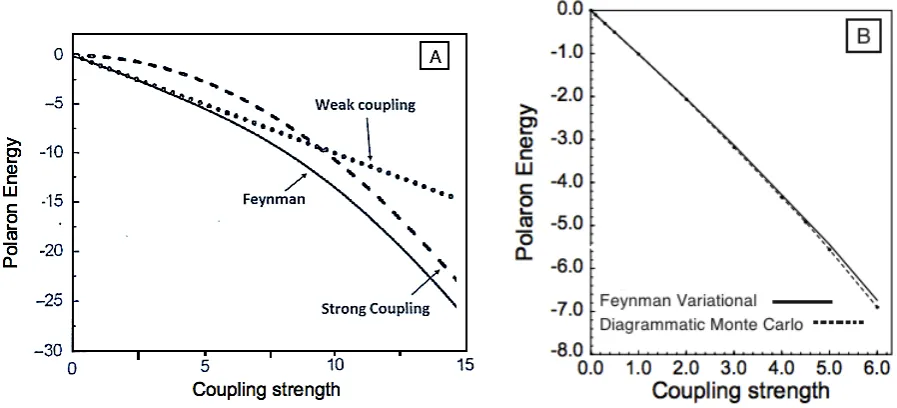
1.2 A) The ground state energy (in units of ~ω0) for the Fröhlich polaron as a

function of the electron-phonon coupling, calculated with the weak coupling, strong coupling and Feynman variational formalism. B) Diagramatic Monte-Carlo (Dashed line) and Feynman variational formalism (Solid line). . . 16

1.3 Representation of the process of an electron with momentum (P−k) and a phonon of momentum k. . . 19

1.4 Velocity distribution of Rb atoms at differents temperatures [1]. The atoms exhibit a Maxwell distribution at 400 nK (left), but at 200 nK a macroscopic fraction of the atoms occupies the state corresponding to velocity zero(center) and for T = 50nK almost all the atoms are in this fraction (right). . . 22

1.5 Representation of the interatomic potential V and the effective po-tential Vef f. The details of the potential for short distances are irrelevant. For large distance both yields the sames−wave scattering length. . . 24

(12)

1.7 Observation of a magnetically tuned Feshbach resonance in an optically trapped BEC of Na atoms. Scattering length normalized to the abg as a function of the external magnetic field B . The resonant point is placed at B0 = 907G. Dots

represents the experimental data, whereas the solid line is the theoretical formula [2]. . . 29

2.1 Fermi Polarons: from polarons to molecules. (a) For weak attraction, an impurity (blue) experiences the mean field of the medium (red). (b) For stronger attraction, the impurity surrounds itself with a localized cloud of environment atoms, forming a polaron. (c)For very strong attraction, molecules of sizea are formed despite Pauli blocking of momentak < kF 6a−1 by the environment. . . 32 2.2 Attractive and repulsive Fermi polarons in 2D: (a) Energy spectrum

displaying the many-body ground state of the system, characterized by both the attractive polaron, the molecular state and the repulsive polaron lying in a metastable branch as a function of the interaction strength written in typical experimental units ln (kFa). The single particle spectral function (b) dis-plays a well-defined pick for weak attractive interactions, thus characterizing the attractive polaron. When the interaction strength is driven near to the reson-ance the pick is not well-defined(c)and the single particle spectral function will display an incoherent feature as soon as the resonance is crossed and enters into the molecular branch (d). . . 33 2.3 Mean results from the Köhl team about 2D fermionic polarons [2.2]:

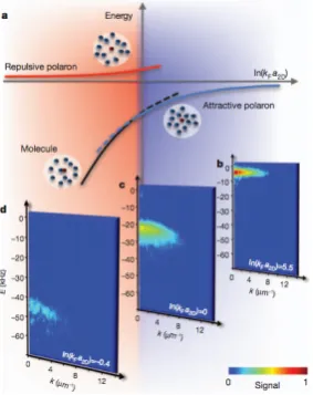
(a)Energy normalized as a function of the strength parameter defined as ln(kFa). Theory [3] and experiments are plotted. (b) The effective mass was investig-ated for both the attractive (red squares) and the repulsive polaron (blue circles) as a function of the strength parameter as well as a (c)function of the temperature and (d) the impurity concentration. All previous results for the effective mass displays non-self trapping for the impurity. The life-time (e) of the repulsive polaron is plotted as a function of the coupling strength. . . 35 2.4 Results from the Grimm team concerning 3D fermionic polarons [2.4]:

similar to the case in two dimensions the energy spectrum displays two polaronic branches as a function of the strength parameter defined here as 1/(kFak−Li):

(13)

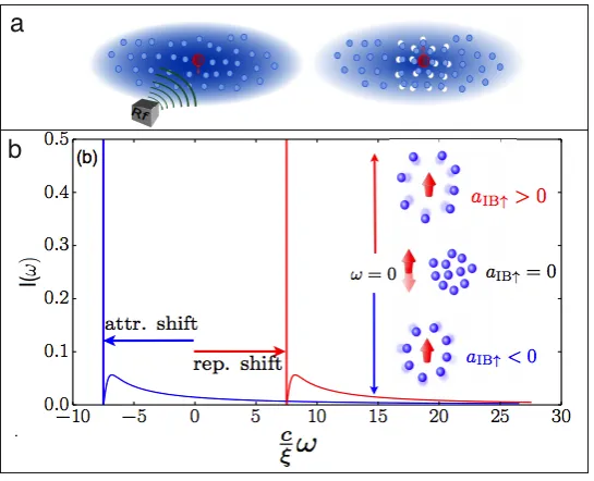
2.5 Radio Frequency spectroscopy (rf) for investigating the spectral properties of a BEC: The mean idea of RF spectroscopy is drive a non-interacting system to a interacting system form two internal states of the impurity (a) a small concen-tration of impurities with two internal levels|↓iand|↑i(red spheres) is immersed

into a BEC (blue spheres), in which the interaction between the impurity-boson is featured by thes−wave scattering length aIB. A radio frequency pulse

trans-fers impurities from a non-interacting state |↓i to a interacting state |↑i. (b) The transition from |↓i to |↑i is made by a coherent well-defined peak centered

at a frequency correspondig to the energy polaron. The picks show up for both attractive (aIB↑ < 0) and repulsive interactions (aIB↑ > 0) . Moreover the

high-frequency power-law tail is associated to the low energy excitations in the BEC. . . 37 2.6 (A) single spin impurity is flipped at the center site of a 1D spin chain. Each

spin is coherently coupled to its neighbors through the superexchange coupling. (B) Quantum evolution of the spins as a function of the time. . . 39 2.7 Experimental array for impurities in a one dimensional gas: (A)

species-selective dipolar potential localizes the impurities into the center of a one dimen-sional Rb atoms. (B) The ultracold Rb atoms with K impurities are loaded into

a one dimensional array.(C) The axial width σ = qhx2_i is plotted as a

func-tion of the time for different ratios η=gK,Rb/gRb displaying the effects of the K

impurities on theRb atoms. . . 39

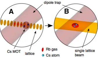
2.8 133_Cs _{atoms are immersed in a ultracold gas of} 87_Rb_{. . . 40}

3.1 Representation of the matrix [3.27]: each column of the matrix is a state where the system lies. In our example we haveN = 4 particles distributed onW walkers. 52 3.2 The ground-state energy per particle is calculated with the SVMC.

Green points represent the SVMC data and orange line represents the linear fitting. The time dependent VMC algorithms [3.4.1] are affected by a time-step bias. By using the SVMC that relies on a transition probabilitity defined by Eq. [3.53] and an acceptance probability given by Eq. [3.54] the time-step dependence is eliminated. . . 59 3.3 Periodic boundary conditions (p.b.c): when a particle (green ) leaves the

box on the left side, a virtual particle (gray) enters the box on the right side. . 59 3.4 Cut off radius r < L/2 for inter-particle correlations. Particle B lies inside the

(14)

3.6 Ground state energy per particle as a function of the iteration number in VMC for a weakly interacting Bose gas with gas parameter (nBa3) = 10−5. Green line direct estimatorED given by Eq. [3.107] and red line, force estimator EF given by Eq. [3.112]. . . 72 3.7 Example of the boson-boson pair correlation function gBB(r): (A) For

short distances, this is related to how the particles are distributed in the sim-ulation box. For example, consider hard spheres (bosons). The spheres can’t overlap (HS potential), so the closest distance between two centers is equal to the diameter of the spheres. Further away, the bosons get more diffuse, and so for large distances, the probability of finding two bosons with a given separa-tion is essentially constant. This is represented by the boson-boson correlasepara-tion function. (B) histogram representing the statistics. . . 74 3.8 SDMC ground-state energy per particle as a function of the time-step:

Forδτ →0 we obtain ED(0 NB)/NB = (1.2617±0.0020)×10−4 _{. . . 76}

3.9 Number of walkers dependence: ground-state energy per particle of a Bose gas with nBa3 = 10−5 as a function the inverse on the number walkers. For 1/NW _→_{0 we obtain a value} _E_D(0 _N_B)_/N

B = (1.2625±0.0010)×10−4. . . 77 3.10 Finite-size effects: ground-state energy per particle as a function 1/NB of a

weakly interacting Bose gas withnBa3 = 10−5. FornB = N_VB_→∞→∞ = constant, one gets ED(0 _NB)_/N

B = (1.266±0.010)×10−4 . . . 77 3.11 Ground-state energy per particle of a Bose gas as a function of

para-meter (nBa3)

1/3_{. Red line from the Bogoliubov theory Eq. [1.34] and green}

points are the DMC simulations. . . 78 3.12 boson-boson correlation pair function as a function of the inter-boson

dis-tance. For a Bose gas with nBa3 = 10−5. . . . 79 4.1 Perturbation of the impurity in the bosonic bath: A)The initial state has

an impurity of momentump and no phonons B) an excited state is represented by the impurity with momentum p+_~k and a phonon with momentum−_~k. . 85 4.2 Variational model for an impurity interacting with a BEC:the impurity

(15)

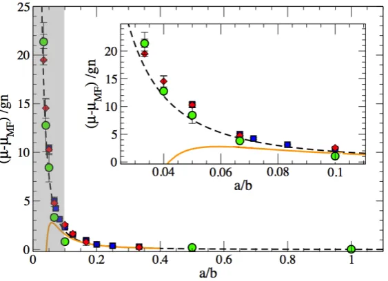
4.3 Reduced binding energy (F =µ−µM F) in units of 4π~ 2_n

Ba

m as a function of the coupling strength a/b computed with perturbation theory (dashed black line), using the Jensen-Feynman variational formalism (solid orange line) and the DMC method for two different ASW potential ranges a/R0 = 5 (filled

green circles) and a/R0 = 20 (filled red diamonds) and the HS potential (blue

square). . . 95 4.4 (A) Binding energy as a function of the strength interaction, for both the

attractive and repulsive branch. In the inset we show the binding energy for a/b > 0 along the attractive branch. The red line shows the two-body binding energy (B) Reduced binding energy as a function of the coupling strength a/b for both the attractive and the repulsive branch. . . 97 4.5 Mean square displacement of the impurity as a function of the

ima-ginary time for the case where the impurity and the bosons do not interact (purple), a/b = −1 (yellow); a/b = −0.2 (blue), a/b = −0.1 (red) and a/b = 0 (green). . . 98 4.6 Effective mass as a function of a/b: perturbation theory (red dashed line),

Jensen-Feynman (solid blue line), DMC simulations with ASW potential (green points). The range of the potential in the DMC simulations isR0 = 0.2a. . . 99

4.7 Boson-boson pair correlation function gBB(r) on the respulsive branch

b

a = +30

(green solid line), at the unitary limit (red solid line) on the attractive branch and for the case where the impurity is absent (blue solid line). . . . 100 4.8 Density profiles n(r) (in logarithmic scale) as a function of the

dis-tance in units of the healing length ξ . The profiles are computed for both the attractive (solid blue line) and the repulsive (green solid line) branches for coupling strengths: b/a=±10,±20 and b/a=±30. The dashed line represents the equilibrium density nB. In the insets the number of bosons as a function of the distance in units of the healing length for the attractive and repulsive branch.101 4.9 Enhacement for the attractive branch (right) and deplection for the

repulsive branch (left) of the density profile.The dashed line represents the equilibrium density nB. . . 102

(16)

5.2 Binding energy as a function of the gas parameter(nBa3)1/3at the unit-ary. Green points represent DMC simulations. . . 105 5.3 Dependence on the binding energy with (nBa3)

1/3

at the unitary limit: Green points stand for DMC, whereas the red line is a power law fitting. . . 106 5.4 Effective mass of the polaron at the unitary limit as a function of the

gas parameter nBa3 of the bosonic bath. . . . 107 5.5 Boson-boson pair correlation function at thea/b= 0for different values

of the gas parameter nBa3. . . . 108 5.6 Density profile (in logarithmic scale) at the unitary limit as a function of the

inter particle distance for different values of nBa3: green (nBa3 = 3x10−6), red (nBa3 = 1x10−5), blue (nBa3 = 1x10−4). Inset: parameterC contact as a func-tion of (nBa3)2/3. The dashed line represents the equilibrium densitynB. . . . . 109 5.7 Total energy in units of _~2_/ma2 _{for a system consisting of two bosons}

and one impurity with resonant interspecies interaction as a function of the inverse of the size of the simulation box a/L. . . . 110 6.1 Generalized binding energy in units of gnBx as a function of b/a along

the repulsive branch for different concentrations x = 3/64, 5/64, 7/64 and x = 9/64. Both perturbation theory (blue dashed line) and DMC results (filled green circles). . . 126 6.2 Generalized binding energy (in units of gnBx ) as a function of b/a for

different concentrations x= 3/64, 5/64, 7/64 and x= 9/64. . . . 126 6.3 Generalized binding energy (in units ofgnBx) once the mean-field term

(µM F) is substracted as a function of b/a for different concentrations x= 3/64, 5/64, 7/64 and x= 9/64.Perturbation theory (blue dashed line) and DMC results (filled green circles). . . 127 6.4 Generalized binding energy in units of gnBN as a function of the

con-centration x. Forb/a =−5 (lower branch) andb/a = +5 (upper branch) com-puted with perturbation theory (blue dashed line), collective variables method (solid red line) and DMC results (filled green circles). . . 128 6.5 Residual function F(x) as a function of the concentration x for both

(17)

6.6 Homogeneous phase: M bosons of type A (green balls) and N bosons of type B (blue balls) immersed in a cubic box of size L. . . 130 6.7 Representation of h1(nBa3, _ab) for differents values of _ab and nBa3. For values of

h1 >0, the homogeneous phase is stable. . . 132

6.8 Phase II: (left) M bosons in the region A and N bosons in the region B distributed in different volumes VA 6=VB. (right) stability of the phase separated state, . . . 132 6.9 Plot of h2(nBa3, _ab) as a function of _ab for different values ofnBa3. For values of

h2 <0, the phase separated state is unstable. . . 134

6.10 Phase diagram for different values ofnBa3 as a function of the coupling strength b/a. The stable homogeneous phase is represented by the green region, whereas the stable phase separated state is represented by the blue region. The horizontal dashed lines represent the interval where perturbation theory works. . . 135

7.1 Bunching data algorithm for a sample of correlated data. Taking from Ref. [4]. . 140 7.2 Bunching data algorithmtaking from Ref. [4]. . . 140 7.3 Estimation of the true error in a DMC simulation for 10000 iterations of the

total energy for a system of bosons in a cubic box. . . 140 7.4 Plotting of Eq. [3.63]. For R0/a = 0.2. By tunning the deep and range of

the ASWP, one can access either to attractive interactions when K0R0 < π/2

(18)

(19)

Chapter 1

Introduction

In this thesis we investigate the properties of an impurity immersed in a dilute Bose gas at zero temperature using quantum Monte-Carlo methods. The interactions between bosons are modeled by a hard sphere potential with scattering length a, whereas the interactions between the impurity and the bosons are modeled by a short-range, square-well potential where both the sign and the strength of the scattering length b can be varied by adjusting the well depth. We calculate the binding energy and the effective mass of the impurity along the attractive and the repulsive polaron branch. In particular, at the unitary limit of the impurity-bosons interaction, we find that the binding energy is much larger than the chemical potential of the bath while the effective mass remains on the order of the bare mass. We characterize the ground state of the impurity by calculating the bosons-boson pair correlation function and by investigating the dependence of the binding energy on the gas parameter of the bosonic bath. Additionally, we present some results concerning the problem of many impurities immersed in a Bose quantum gas by using both perturbative and Monte-Carlo methods.

(20)

ground-state energy.

In the second chapter we provide a review of experiments concerning impurities immersed in quantum gases. We briefly discuss the Fermi polaron, which consists in a dressed spin-down impurity in a Fermi sea of spin-up particles. The Fermi polaron displays an energy spectrum formed by two branches: a metastable repulsive and the ground-state attractive branch. The metastable polaron may decay eventually into the attractive branch consisting of a molecular state formed by the impurity and a particle from the Fermi sea. Various properties, such as the polaron effective mass and lifetime, are investigated experimentally. The Fermi polaron are observed both in two and three dimensions. In the second part of the chapter we summarize some experiments concerning impurities immersed in a Bose gas. We start with experiments in one dimensional systems where the dynamics of a single impurity is studied. Properties such as the energy and the effective mass are investigated as a function of the coupling strength between the impurity and the bosonic bath. At the end of the chapter we mention an important experiment that could be linked to our project: the dynamics of neutral impurities immersed in an ultracold Bose gas in three dimensions.

The third chapter is devoted to develop the concepts of the Quantum Monte-Carlo (QMC) methods. These are techniques I used to study the problem of the polaron immersed in a degenerate Bose gas at zero temperature. We start by mentioning the importance of the com-putational methods compared to more analytical tools in the regime of strong correlations and we explain some preliminary concepts such as: random variables and stochastic processes and how observables are calculated in QMC techniques, in particular energy, correlation functions and effective mass of an impurity. The specific techniques that I used are them introduced: the Variational Monte-Carlo (VMC) and the Diffusion Monte-Carlo methods (DMC). The technical details are explained for both methods and the chapter closes with a case study: the calculation of the ground-state energy for a Bose gas as a function of the gas parameter.

(21)

devised using a variational principle. The Jensen-Feynman free energy approach allows one to calculate the ground-state energy for the impurity problem immersed in a Bose gas for all the values of the coupling strength. A functional action can be written using the Fröhlich’s Hamiltonian; then this action is introduced into the Jensen-Feynman inequality and the free energy of the system is obtained by a minimization procedure. Furthermore, the effective mass of the impurity is calculated using this technique. We then address the problem using QMC methods. In particular, the Diffusion Monte-Carlo technique is used to study the ground-state properties of the bath-impurity system. This system is characterized by N bosons plus one impurity in a cubic box with periodic boundary conditions. We calculate the binding energy of the impurity defined as the difference of the ground-state energy E(N + 1) of the system plus the impurity and the ground-state energy E0(N) of the system without impurity. Similarly to

the Fermi polaron problem, we find two branches: a repulsive and an attractive branch corres-ponding to effective repulsive and attractive interactions between the impurity and the bath. We compared the polaron binding energy with the mean-field results obtained at the beginning of the chapter. In the weak-coupling regime the polaron binding energy is obtained with both pertubative and variational methods are in good agreement with the QMC results, however significant differences appear at strong coupling. In addition, both the boson-boson and the impurity-bosons correlation functions are calculated for all values of the coupling strength, in order to understand the effects of the impurity on the bosonic bath when the interaction is either attractive or repulsive. The effective mass has been computed by using QMC techniques and agreement is found with mean-field results in the weak-coupling regime. In the strongly interacting limit we find a finite value of the effective mass. This is in contrast with the results of the mean-field methods where the effective mass is predicted to diverge and self-localization of the impurity is claimed.

The fifth chapter treat separately the regime of strongest coupling between the impurity and the Bose gas known as the unitary limit. We investigate the dependence of the binding energy with the gas parameter. At low densities the binding energy is much larger than the chemical potential of the bath. On the other hand, the effective mass is found to reach a value around twice the bare mass of the impurity. The chapter closes by investigating the possible existence of a three-body bound state in our model.

(22)

Figure 1.1: The ions placed on the lattice fell the attraction by the electron, therefore there is a distortion of the lattice. This electron and this distortion can be described by a quasi-particle with different mass and energy respect the naked electron and this quasiquasi-particle is called polaron.

strengthb/a.

At the end of the thesis some conclusions and remarks are drawn form the theoretical point of view. In addition we will discuss some interesting features about possible experimental realizations of impurities immersed in a bosonic bath.

1.1

Fröhlich solid-state polaron

In this section, we turn our attention to the polaron problem in solid-state physics. In this context, a central problem is the study of electrons and phonons and their interactions. When an electron at rest or in movement interacts with the ions placed in the lattice, then the negative charge of the electron will attract the positively charged ions and repel the negatively charged ones Fig [1.1]. The electron together with its self-polarisation cloud will form a new quasiparticle called polaron. The energy and the mass of this quasiparticle are different from the bare electron.

The concept of polaron was introduced by Landau and Pekar [5] in 1933. The distortion of the lattice can be described in terms of phonons. The Fröhlich Hamiltonian derived by Fröhlich [6] in 1954 describes the interaction between electrons and the longitudinal optical phonons (LO) due to the lattice distortion. The Hamiltonian can be written as:

H=X

p P2 2Mˆc

˙

†

pcpˆ +

X

~ωqˆa†qˆ˙aq+X

q,p

Vqˆc†p˙+qˆcp

ˆ

(23)

deeply discused in Reference [7]. The first term in Eq. [1.1] represents the kinetic energy of the unperturbed electrons with momentum P and mass M. The second term is the energy of the phonon bath. The last term describes the interaction between optical phonons and electrons in terms of a k−dependent Vk. The particular case of just one single electron reduces the

Hamiltonian Eq. [1.1] to:

H=P

2

2M +~ω0

X

q ˆ a†qˆ˙aq+

X

q

Vqexp(iq·r)

ˆ a†_q+ ˆaq

. (1.2)

where the longitudinal phonons are described by the Einstein model with frequency ω0 and

the interaction amplitude between electrons and phonons is given by Vq = M0 ν1/2

1

|q|, ν being the

volume, M₀2 = 4πα~(~ω0)3/2

(2M)1/2 and α = e2

~

M

2~ω0

1/2

1

ε∞ −

1

ε0

where ∞ and 0 are the static and

high-frecuency dielectric constant respectively and depend on the specific material. Then the Hamiltonian Eq. [1.1] is reduced to:

H =P

2

2M +ω0

X

q

a†_q˙aq+

X

q M0

ν1/2

exp(iq·r)

|q|

a†_q˙ +aq

. (1.3)

A couple of features must be pointed out: the result above is obtained independently of the statistics of the particle and the model assumes that the motion is isotropic in space and the energy bands are nondegenerate.

However ifωqis kept general in Eq. [1.1], this Hamiltonian describes in general the problem of a particle with massM coupled to a bath of bosons with dispersion relationωq, mediated through an interaction amplitudeVq. Aside from the optical phonons studied in solid-state physics and described by the Hamiltonian Eq. [1.3]; the electron-phonon interaction can be mediated by acoustical phonons as well, which are known as acousto-polarons or piezo-polarons [8, 9]. Other examples are the ripplon-polarons which consist of one electron on a Helium film and the excitations of the system are described by surface waves called ripplons [10, 11, 12, 13]; the plasmaron is a quasiparticle arising from the strong interaction between plasmon and electron, the plasmaron is a quasiparticle formed by quasiparticle-quasiparticle interactions [14, 15, 16]. When a photon is absorbed by a semiconductor an exciton is formed. This quasiparticle is represented as an excitation of an electron from the valence band into the conduction band. [17, 18, 19]. A more general case are the polaritons. These are quasiparticles resulting from strong coupling of electromagnetic waves with an electric dipole-carrying excitation.

(24)

Figure 1.2: A) The ground state energy (in units of~ω0) for the Fröhlich polaron as a function of

the electron-phonon coupling, calculated with the weak coupling, strong coupling and Feynman variational formalism. B) Diagramatic Monte-Carlo (Dashed line) and Feynman variational formalism (Solid line).

the ground-state energy and the effective mass of the polaron as a function of the coupling parameter between the electron (impurity) and the lattice vibrations (bosons); this method was applied for the first time by Fröhlich [6]. The Brillouin-Wigner and Rayleigh-Schrödinger perturbation theory are introduced as predecessors of the modern formulation of the Green’s function formalism and the properties of the electron are described in terms of the spectral function. The latter is obtained from the self-energy contained in the phonon-electron Green’s function. Both theories are linked directy with the T− matrix theory and the reaction matrix

theory. Both the ground-state energy of the electron and its effective mass are calculated. These methods are described in large detail in Ref. [7].

(25)

In Fig. [1.2] the ground-state energy of the electron (impurity) is calculated for different coup-ling strengths. In Fig. [1.2, A] the ground-state energy is plotted for the weak-coupcoup-ling formal-ism (e.g perturbative methods), the strong-coupling regime (e.g Landau-Pekar strong coupling theory) and the Feynman variational formalism which reproduces very well the weak-coupling limit and provides an upper bound in the strong-coupling limit. Furthermore it interpolates between the two regimes. The strong-coupling regime has been widely investigated with dia-grammatic expansions, where Feynman diagrams are drawn and sampled using Monte-Carlo methods. This method is know as Diagrammatic Monte-Carlo (DiagMC). In Fig. [1.2, B] both results of Feynman variational formalism and Diagramatic Monte-Carlo methods [24, 25, 26] are shown for all values of the coupling strength and they are in good agreement. The DiagMC method is the most powerful tecnnique describing the strong-coupling regime.

The problem of two and more impurities has been widely investigated as well. In particular, an extention of the Feynman variational formalism was developed for two electrons [27]. This study shows that if the polaronic coupling strength is large enough the impurities will form a bound state of two electrons with weak effective Coulomb interaction (the bipolaron). [28]. Under certain circumstancesthe formation of multipolaron are linked with clusters of polarons [29].

In the subsequent section, we will derive the Fröhlich Hamiltonian describing the phonon-electron interaction and a perturbative calculation will be presented in order to estimate both the energy and the effective mass.

1.1.1

Perturbative treatment

In this section we will treat the problem of one electron interacting with the lattice vibrations by means of perturbative methods. One assumes that the electron interacts with the lattice and therefore there is a periodic potential acting on the electron. The lattice is displaced from its equilibrium position and there is a potential ∆V1(x) “ felt” by the electron due to the change

of the charge density ρ(x). This statement is contained in the Poisson equation:

∇2_∆_V

1(x) =eρ(x) = −∇ ·P(x). (1.4)

Let us suppose that the lattice is formed by a postitive and a negative ion placed in each unit cell. Then, there are six total modes for eachknumber. Three of the modes are characterized by the ions moving in the same direction; ask→0 such modes do not provide important contributions

(26)

negative ions produce a polarization that is proportional to the amplitude of the mode (optical branch). For these modes, a gap is present in the excitation frecuency ω0 6= 0 for k →0.

Let us consider ˆa†(k) and ˆa(k) the creation and annihilation operators of phonons respectively. The polarization can be written as:

P(x) = α0

Z _d3k

(2π)3 3

X

i=1

h

ˆ

ai(k) exp (ik·x) ˆek,i+ â†_i(k) exp (−ik·x) ê∗_k,ii (1.5) Where êk,i (ê∗k,i) is the unitary polarization vector (and its complex conjugate) in the direction k. The polarization P(x) is proportional to the net displacement of the ions. In fact the previous equation is obtained by the quantization of the harmonic oscillations of the crystal (see for instance [21]). The proportionality constant isα0 and it depends on the material. From Eq. [1.4] and Eq. [1.5] the charge density is then given by:

eρ(x) = −∇ ·P(x) =iα0

Z d3k

(2π)3 3

X

i=1

h

ˆ

ai(k) exp (ik·x)k·ˆek,i−ˆa

†

i(k) exp (ik·x)k·eˆ

∗

k,i

i

.

(1.6) Evidently the longitudinal mode paralell to ˆek,i has a non-zero contribution (ˆek,i||k). It turns out that

ρ(x) =iα0

Z _d3k

(2π)3k

h

ˆ

akexp (ik·x)−ˆa_k† exp (−ik·x)i. (1.7) The potential energy of the electron due to the lattice vibration can be obtained as

∆V1(x) = −ieα0

Z d3k

(2π)3

1 k

h

ˆ

akexp (ik·x)−ˆa

†

kexp (−ik·x)

i

(1.8)

=i√2πα1/2 ~

5_ω3

M

Z d3k

(2π)3

1 k

h

ˆ

akexp (ik·x)−ˆa

†

kexp (−ik·x)

i

,

where α0 = √2πα1/2(_~5_ω3_/M₎1/4 _, _α ₌ 1 2 1 ε∞ − 1 ε0 e2 ~ω

2M ω ~

1/2

and ε∞, ε0 are the static

and high-frequency dielectric constants of the crystal respectively. The total Hamiltonian reads as

H=P

2

2 +

X

k ˆ

a†_kaˆk+i

√

2πα1/2X k

1

|k|

ˆ

a†_kexp(−ik·r)−ˆakexp(ik·r)

, (1.9)

(27)

Figure 1.3: Representation of the process of an electron with momentum (P−k) and a phonon of momentum k.

estimate the energy of the polaron. Therefore, one assumes a perturbative parameter, in this case the coupling constant α1.

In perturbation theory one splits the Hamiltonian Eq. [1.9] as H=H0+Hpert , where

H0 = P 2 2 +

P

kaˆ

†

kˆakand

Hpert=i

√

2πα1/2P 1

|k|

ˆ

a_k†exp(−ik·r)−akˆ exp(ik·r), (1.10) and the energy is written as a perturbative expansion, namely:

∆E0 =h0|Hpert|0i+

X

n

h0|Hpert|ni hn|Hpert|0i E0

0 −En0

+· · ·

As it is standard in perturbation theory, |ni and En are the eingenvectors and eigenvalues of

H0 respectively. Since Hpert acting on a state changes the number of phonons, the first term of the perturbative series vanishes.

In the Fig. [1.3] the initial state is represented by an electron with momentum P and no phonons. In an intermediate state the electron has a momentum (P−k) and there is one phonon emitted. Therefore the energies of these states are:

Initial state : E₀0 = P

2

2 . (1.11)

Intermediate state : E_n0 = (P−k)

2

2 + 1. (1.12)

(28)

is given by:

hn|Hpert|0i=i

√

2πα1/2

* n X k 1

|k|

ˆ

a†_kexp(−ik·r)−ˆakexp(ik·r)

P, no phonons

+

.

(1.13) It vanishes unless|niis a state with one phonon and one electron with momentum P0, namely

|ni=|P0, 1phononi. If the phonon has momentum k, it turns out that,

hn|Hpert|0i=i

√

2πα1/2

*

P0, no phonons

1

|k|exp(−ik·r)

P, no phonons

+

. (1.14) Since exp(−ik·r)|Pi=|P−ki,P0 =P−kis expected by the momentum conservation. Then

hn|Hpert|0i=i

√

2πα1/2 1

|k|δp0,p−k, (1.15)

∆E0 =−

√

2παX k

1

|k|2

1

(P−k)2_/2 + 1₋_P2_/2 ×2

!

. (1.16)

The factor 2 in the previous expression is due to the spin of the electron. By writting the sum as an integral using P

k=V

R d3_k

(2π)3 it turns out

∆E0 =−2

√

2πα

Z d3k

(2π)3_|_k_|2

2

k2₋2_P_·_k+ 2

. (1.17)

The integral is computed using the fact thatR d3k/(2π)3

|k2₊_a_|2 = 1

8π√a. Adding both the kinetic energy and the second order corretion of the energy, one obtains

E = P

2

2 −α− p2

12α+· · ·=

P2

2 (1 +α/6) −α+· · · (1.18) As it can be inferred from the previous equation the electron mass is increased due to the polarisation of the media. The polaron is described as a free particle with m∗/m= 1 +α/6 . Experimentally in the solid state context, both weak and intermediate coupling regimes have been tested and they are in good agreement with the theoretical approaches mentioned in this chapter [30, 31]. Nevertheless, there are materials with large values of the coupling parameter where perturbative theories are not longer adequate.

(29)

1.2

Ultracold gases and Bose Einstein consensates

The first ideas of Bose Einstein condensation (BEC) appeared in 1925 when A. Einstein expan-ded the ideas of S.N Bose about the quantum statistics of light quanta (now called photons) [32]. Einstein considered a non-interacting system of massive bosons and he established that below a certain critical temperature, a large finite fraction of bosons would occupy the lowest-energy single-particle state [33]. In 1938, after the discovery of the superfluidity in liquid 4He

[34], F. London suggested that there was a connection between superfluidity and Bose Einstein condensation [35]. The first theoretical explanation of superfluidity was provided by Landau in 1941 [36] in terms of the elementary excitations of the fluid. Later on, Bogoliubov de-veloped the first microscopic approach in order to describe an interacting Bose gas [37]. In 1951 simultaneously Landau and Lifshitz [38] and Penrose [39] realized that there was an in-trinsic relation between the one-body density matrix and the macroscopic occupation of the single particle state where bosons are condensed. The concept of non-diagonal long-range order came out as a key point in order to understand BEC. This concept was also helpful in order to make the link between superfluidity and BEC clearer [40]. On the other hand, Landau’s predictions concerning the excitation spectrum in superfuid 4He were verified experimentally.

Furthermore the momentum distribution was measured for the superfluid 4He yielding

inform-ation about the condensed fraction. Starting, from the experimental observinform-ations about the specific heat in superfluid 4_He [41] Landau proposed the existence of a quasiparticle named

roton, that is an elementary excitation in the fluid, responsible of the behaviour of the specific heat. After, the theoretical prediction of quantized vortices by Onsager [42] and Feynman [43] were experimentally confirmed by Hall and Vinen [44].

In 1970, many experimental techniques aiming at the study of atomic physics appeared; such techniques are based on magnetic and optical trapping. In the 1980’s laser-based techniques, such as laser cooling and magneto-optical trapping were developed for cooling and trapping neutral atoms [45, 46, 47]. Furthermore, alkali atoms were found as very suitable candidates in the laser-based methods, since their optical transitions can be excited by a laser and their internal energetic structure allows one to cool them to low temperatures (a theoretical descrip-tion of trapping and cooling of atoms can be found in chapter 4 of Ref. [48]). Once atoms are trapped their temperature can be lowered further by using evaporative cooling. Finally, in 1995, by using the evaporative cooling techniques, Bose Einstein condensation was achieved for dilute atomic gases of 87_{Rb atoms by Cornell and Wieman at Boulder [1] and simultaneously}

by Ketterle at MIT using 23_{Na atoms [49]. The different species were cooled down to very}

low temperatures on the order of fractions of µK. In the same year Bradley and colleagues achieved BEC of7Li [50, 51]. Since then, BEC was achieved in many other atomic species such

(30)

Figure 1.4: Velocity distribution of Rb atoms at differents temperatures [1]. The atoms exhibit a Maxwell distribution at 400 nK (left), but at 200 nK a macroscopic fraction of the atoms occupies the state corresponding to velocity zero(center)and forT = 50nK almost all the atoms are in this fraction (right).

are not the unique species displaying BEC: it has been achieved with ytterbium isotopes [56], strontium [57], and erbium atoms[58] as well as with molecules [59, 60].

It is very convenient to observe and analyze BEC’s in dilute cold gases. The experiments are very clean and the basic theoretical description is much less involved than in traditional condensed-matter systems such as superfluid 4He. Diluteness and low temperatures are the

main features of these cold gases.

Diluteness: Let us consider a gas of bosons of mass m and density nB = NB/V. Where NB is the number of bosons and V the volume. In a dilute homogeneous gas the range R0 of

the interatomic forces is much smaller than the average distance between particles; namely d=n−_B1/3. In other words,

nBR03 1. (1.19)

In fact, in alkali atoms interacting via a van der Waals potential, the typical range of the inter-actions is around two orders of magnitude greater than the size of the atoma0 (the Bohr radius)

and is much smaller than the typical interparticle separation ∼ 103_a

0 [48]. Corresponding to

typical densities ranging from 1013_/cm3 _{to 10}15_/cm3_.

(31)

derived from the diluteness condition establishes that pair collisions are well described by a single parameter, the s−wave the scattering length [48]. All the properties of the system are

described in terms of this parameter and do not depend on the specific details of the two-body potential (see. Section 1.2.1).

Low temperatures: BEC is achieved for temperatures lower than a critical temperature KBTc = 2π~

2 m

_n B

2.612

2/3

, with m the mass of the bosons [61]. In fact, the thermal de Broglie wavelength Λ = h/√2πmKBT for massive particles must be on the order of the interparticle distancenBΛ3 _∼1_. In addition if

ΛR0, (1.20)

the scattering amplitude becomes independent of the collisional energy as well as of the scat-tering angle and a low-energy approximation can be used. According to the scatscat-tering theory at low energy, this scattering amplitude is determined by the s−wave scattering length which

characterizes the effects of the interaction without specific knowledge of the potential details. The condition of diluteness Eq. [1.19] can be re-written in terms of the s−wave scattering

length as:

nB|aBB|3 1. (1.21)

If a quantum gas satisfies the condition [1.21], mean-field theories are suitable for its theoretical description. On the contrary, if the gas parameter is not small enough the system is no longer weakly interacting and other tools must be used, e.g beyond mean-field tecniques or quantum Monte-Carlo methods.

In section [1.2.1] we will discuss the scattering length and how it can be tuned in order to change the interaction between atoms. Before let us calculate the ground-state energy of a dilute Bose gas at low temperatures using the Bogoliubov mean-field approach.

The Hamiltonian for a uniform dilute gas of bosons is written in the form:

H =X

p p2

2mˆa

†

pˆap+ 1 2V

X

p1,p2,q

Vqâ†_p₁₊qâ†_p₂−qâp1âp2, (1.22)

with Vq =

R

V(r) exp [−iq·r/_~] dr, the Fourier transform of the interatomic potential. In real systems, for instance 4_{He, interaction can be modelled by a two-body potential. However, in}

(32)

Figure 1.5: Representation of the interatomic potential V and the effective potential Vef f. The details of the potential for short distances are irrelevant. For large distance both yields the same s−wave scattering length.

the q = 0 component of the Fourier transform of the effective potential :

V0 =

Z

Vef f(r)dr (1.23)

Then the Hamiltonian Eq. [1.22] is written as:

H=X

p p2

2mˆa

†

pˆap+ 1 2V V0

X

p1,p2,q

ˆ a†p1+qˆa

†

p2−qˆap1aˆp2. (1.24)

In the Bogoliubov approximation one makes the crucial substitution ˆa0 →

√

N0. For an ideal

Bose gas at zero temperature the occupation number for p6= 0 vanishes because all the atoms

are in the condensed stateN0 =N. In a dilute gas the occupation number for states withp6= 0

is finite but small. To lowest order, it is plausible to neglect all the terms in the Hamiltonian containing terms withp6= 0 and therefore ˆa0 ≡

√

N0 =

√

N. Within these approximations the ground-state energy is given by

E0 =

N_B2

2V V0. (1.25)

As it was mentioned before, the two-body potential merely depends on the scattering length aBB. In fact,V0 = (4π~2/m)aBB is obtained by using the Born approximation (See Sec [1.2.1]). The ground-state energy can be written in terms of the coupling strengthgBB = (4π_~2/m)aBB:

E0 =

1

2gBBnBNB. (1.26)

By computing the total pressure for the interacting gas one obtains P = −∂E0 ∂V =

gBBn2_B

2 ,

(33)

computing the compressibility of the gas one obtains κ = ∂nBB

∂P =

1

gBBnBB. Thermodynamic

stability requires that κ > 0 and therefore a weakly interacting Bose gas is stable if aBB > 0 (repulsive interactions).

The ground-state energy in Eq. [1.26] has been derived within the lowest-order mean-field approach. Higher-order approximation scheme can be used where quantum fluctuations are included.

In order to go beyond the lowest-order mean-field approximation, one must consider two aspects: 1. Quadratic terms are considered in the operators withp6= 0 , thus the Hamiltonian in Eq.

[1.24] turns out to be:

H =X

p p2 2mˆa

†

pˆap+ 1 2V V0aˆ

†

0â†0â0â0 + 1 2V V0

X

p6=0

4â†₀aˆ†pâ0âp+ â†pâ

†

−pâ0â0+ â

†

0ˆa†₀aˆ0ˆa−p

(1.27) 2. The higher-order Born approximation must be considered for the relation between the

potential V0 and the scattering length aBB. This givesaBB is calculated as [62]:

aBB = m 4π_~2



V₀+

V₀2 V

X

p6=0 m p2



. (1.28)

One should point out that the Hamiltonian in Eq. [1.27] can be rewritten by the equation for number of particles N = â†0â0+Pp6=0â†pâp yielding:

ˆ

a†0â†₀â0â0 =N2−2N

X

p6=0 ˆ

a†pˆap. (1.29)

By plugging Eq. [1.29] and Eq. [1.28] into Eq. [1.27] one ends up with:

H= gBBN

2

B 2V +

X

p p2 2mˆa

†

pˆap+ gBB

2 nB

X

p6=0

2â†_paˆp+ â†pâ

†

−p+ ˆapˆa−p+

mgBBnB p2

!

. (1.30)

The previous Hamiltonian is quadratic in the operators ˆa†_p and ˆap and it can be diagon-alized using the Bogoliubov transformation, where operators are written in terms of a set of new operators ˆαp and ˆα†p. By following Bogoliubov’s procedure [37] the diagonalized form of the Hamiltonian is

H=E0+

X

p

(p)ˆα†_pαˆp, (1.31) here

E0 =

gBBN_B2 2V +

1 2

X

p6=0

(p)−gBBnB− p2 2m +

mg2_BBn2_B p2

!

(34)

and the dispersion relation(p) is given by:

(p) =

v u u t

gBBnB

m p

2+ p 2

2m

!2

. (1.33)

The Bogoliubov transformation allow us to map a weakly-interacting system into a system of independent quasiparticles with energy(p). The operators ˆαp and ˆα†_p are the annihilation and creation operators of these quaseparticles. In fact, ˆαp|Vacuumi= 0 defines the ground state

of the interacting system as the vacuum of quasiparticles. Eq. [1.32] gives the ground state energy E0 after substituting the sum by an integral

_V

(2π)3

P

k →

R

d3_k_{. The result is given by}

E0 =

gBBNB2 2V

"

1 + ₁₅128√

π

nBa3BB

1/2 #

, (1.34)

where the lowest-order mean field ground-state energy Eq. [1.26] is now corrected by the Lee-Yang-Huang term [63]. The previous result is valid provided that nBa3BB 1.

We refer to ˆαp|Vacuumi= 0 and to Eq. [1.34] as the equation providing the ground-state and the ground-state energy of the system. Actually the true ground-state of the system is a solid and the gas phase can be observed as a metastable phase where thermalization is ensured by two-body collisions and extremely rare events three-body collisions.

1.2.1

Interatomic interactions and Feshbach resonances

In the previous section thes−wave scattering length was introduced. It characterizes the

low-energy interactions between pairs of particles. The wave function for the relative motion of two colliding atoms can be written as the sum of an incoming plane wave and a scattered wave

ψ(r) =eikz +ψsc(r). (1.35)

One is interested in the behavior of the scattered wave for distances r R0. Under the

assumption that the interaction between particles is spherically symmetric. It turns out to be a spherical wave ψsc(r R0)→ f(θ) exp (ikr)/r, where f(θ) is the scattering amplitude which

depends on the scattering angle θ, that is the angle between the direction of the momentum of the particles before and after the collision. As it was argued before, at very low energies only the s−wave scattering is important. In this limit the wave function displays the asymptotic

behaviour

ψ(r) = 1− a

r, (1.36)

(35)

In what the follows we will see how the knowledge of the scattering length is enough to describe the interaction between pairs of atoms at low energies. There is a connection between the scattered wavefunction ψsc(r) in Eq. [1.35] and the scattering T matrix. The latter satisfies the so-called Lippmann-Schwinger (LS) equation (see Ref. [48]).

T(k,k0;E) =U(k,k0) + 1 V

X

k00

U(k0,k00) E−~

2

mk

00₊

iδ

!−1

T(k00, k;E), (1.37) where U(k,k0) is the Fourier transform of the bare atom-atom interaction. T(k,k0;E) is the defined in terms of the scattered wave function in the momentum space as:

ψsc(k0) = ~

2_k2

m −

~2k02

m +iδ

!−1

T(k,k0;E), (1.38) and k and k0 are the momentum of the incoming and outgoing wave respectively. The value δ in the previous equation is introduced to ensure that only outgoing waves are present in the scattered wave. At large distances for zero energy Eq. [1.38] yields:

ψsc(r) = m

4π_~2_rT(0,0,0) (1.39)

Therefore, it follows that

T(0,0,0) = 4π~

2

m a (1.40)

An approximation for a can be obtained using the Born approximation. It is obtained by ccoinciding the first term on the right-hand of Eq. [1.37] and yields:

a= m

4π_~2V(0) =

m 4π_~2

Z

drV(r), (1.41)

For very low-energies, two body interactions in ultracold gases may be described by a pseudo-potentialV(r) with the scattering lengthataken as an experimental parameter. The scattering length can be either positive or negative corresponding to attractive and repulsive interactions respectively. We now mention how the scattering length can be varied experimentally in order to adjust the interaction between atoms.

(36)

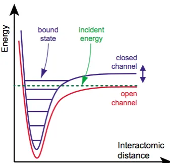
Figure 1.6: Basic two-channel model for a Feshbach resonance: two atoms colliding with energy E (dashed green line) in the open channel (red line) corresponding to the interaction potential is resonantly coupled to a closed channel (purple line). Then a bound state appears on the closed channel with an energy close to zero. The position of the closed channel can be changed with respect to the open channel by varying the magnetic field.

instance, they may correspond to different hyperfine states of the atoms. Feshbach resonances permit tuning of the scattering length by changing a magnetic field [65]. The tunability arises from the difference between the magnetic moments of the close and open channel. In fact, the position of the bound state in the closed channel changes with respect to the open channel by varying an external magnetic field.

Experimentally, the scattering length depends on the external magnetic field according to

a(B) =abg 1− ∆B B −B0

!

, (1.42)

Here abg is the off-resonant background scattering length, in the absence of the coupling with the closed channel,B0 is the magnetic field where the resonance appears, ∆B is the resonance

width. For instance, one can consider a collision of two 6Li atoms: they are prepared in the

lowest hyperfine state |↑i = |ms =−1/2, mI = 1i and |↓i = |ms= 1/2, mI =−1i and the magnetic-field dependence of the scattering length for this collision is shown in Fig. [1.7] where the resonance is atB0 = 834 G.

(37)

Figure 1.7: Observation of a magnetically tuned Feshbach resonance in an optically trapped BEC of Na atoms. Scattering length normalized to theabg as a function of the external magnetic field B . The resonant point is placed at B0 = 907G. Dots represents the experimental data,

whereas the solid line is the theoretical formula [2].

chapter breaks down and more sophisticated theoretical tools must be employed.

(38)

(39)

Chapter 2

Impurities and ultracold gases

In this thesis we investigate the ground-state properties of impurities immersed in a bosonic bath. Ground-state properties such as the energy, the pair correlation function and the effective mass. Precisely these properties have been measured and investigated in Fermi polarons. These quasiparticles are found when particles are immersed in a fermionic bath. Nevertheless, since the matter of this thesis is purely theoretical, we warn the lector that the scope of this chapter is a review of the main experiments concerning impurities in ultracold gases. The motivation of this chapter is to familiarize the lector with experimental activity in this field.

In the first part of the chapter, we review the experiments concerning the Fermi polaron, in which ground-state properties such as energy and effective mass are investigated. Subsequently, we review some experiments concerning the manipulation and control of impurities in a Bose-Einstein condensate as well as the polaronic behavior displayed for impurities in one dimensional configurations.

2.1

Fermi Polarons

(40)

Figure 2.1: Fermi Polarons: from polarons to molecules. (a)For weak attraction, an impurity (blue) experiences the mean field of the medium (red). (b) For stronger attraction, the impurity surrounds itself with a localized cloud of environment atoms, forming a polaron. (c) For very strong attraction, molecules of size a are formed despite Pauli blocking of momenta k < kF 6 a−1 by the environment.

In the context of ultracold atoms, both repulsive and attractive polarons are predicted to occurr when a particle interact with a degenerate quantum gas. The attractive Fermi polarons have been the first observed: dressed spin-down (up) impurities in a spin-up (down) Fermi sea of ultracold atoms [73]. Experimentally, a remarkable feature of the polaron is a narrow peak in the impurity radio-frequency spectrum that emerges from a broad incoherent background. The fermionic polaron lies in the framework of two fundamental problems in quantum many-body physics: the crossover between a molecular BEC and a superfluid BCS (Barden-Cooper-Schrieffer) pairing with spin-imbalance for attractive interactions [74] and Stoner’s itinerant ferromagnetism for repulsive interactions [75].

The first experimental evidence of fermionic polarons came out from the group of Zwierlein and colleagues in 2009. They used a spin-polarized cloud of 6Li spin-up (_↑) atoms in the lower

hyperfine state |1i confined in a cylindrically symmetric optical trap in 3D. Then, the spins of

a small fraction of atoms are flipped by using a two-photon Landau-Zener sweep into the state

|3i (spin-down ↓). The polaron energy and the quasiparticle residue for various interaction

strengths around a Feshbach resonance have been found with rf spectroscopy. There is a characteristic peak that becomes more pronounced at the unitary limit 1/kFa = 0 (kF is the Fermi vector andais the scattering length). The energy of the peak as well as the quasiparticle residue functionZ have been measured [73].

The spin-down impurities are immersed in a degenerate Fermi gas of about 5 ×106 _atoms

in the state |1i at a temperature of tenths of the Fermi temperature. For weak interactions

(41)

Figure 2.2: Attractive and repulsive Fermi polarons in 2D: (a)Energy spectrum display-ing the many-body ground state of the system, characterized by both the attractive polaron, the molecular state and the repulsive polaron lying in a metastable branch as a function of the inter-action strength written in typical experimental units ln (kFa). The single particle spectral function (b) displays a well-defined pick for weak attractive interactions, thus characterizing the attractive polaron. When the interaction strength is driven near to the resonance the pick is not well-defined (c)and the single particle spectral function will display an incoherent feature as soon as the resonance is crossed and enters into the molecular branch (d).

shifted away from the mean field result. This polaronic state is stable up to a critical value at strong interactions 1/kFa ' 1 where the impurity will bind one spin-up atom from the environment forming a tightly bound state Fig. [2.1, c]. Then, the new molecular state forms a bosonic dressed impurity.

After the work carried out by the experimental group of Zwierlein team at the MIT, many theoretical approaches have investigated the Fermi polaron with repulsive interactions [76]. The experimental realization of these polarons faced a huge challenge since the strong interactions between atoms sustains a deeply molecular bound state into which the atoms can decay. In 2012 simultaneously the group in Cambrigde led by Köhl and the group of Grimm in Innsbruck succeeded in the realization of the repulsive Fermi polaron. The essential point for studying Fermi polarons is because the Fermi surfaces of the two components in a spin-imbalanced gas are mismatched and bring to light many interesting features.

The Fermi polaron has been studied by Köhl [77] both for attractive and repulsive interactions in two dimensions. They prepared a quantum degenerate gas of 40_{K atoms in a strongly}

imbalanced mixture with an impurity concentration C = a/b of the two lowest Zeeman state a=|F = 9/2, mF −9/2iand b=|F = 9/2, mF −7/2i at low temperatures.

(42)

(blue solid line). For strong enough interactions, the attractive polaron decay into this dimer state. In contrast, in the case of an impurity interacting repulsively with the fermionic bath, the strong interaction between the impurity and the bath can be only achieved if the under-lying interaction potential is attractive, which implies a two-particle bound state. Therefore the repulsive polaron branch (red dashed line) is metastable and these excitations can decay either into the attractive polaron or the molecular state. The single-particle spectral function have been measured as shown in Fig. [2.2, b] and for weak attractive interactions a sharp peak appears revealing the existence attractive polaron as a well defined quasiparticle.