18MAB203T-U2-Book.pdf

(1)

18MAB203T-Probability and Stochastic Process

As per 2018 Regulations of SRM

S. ATHITHAN

DEPARTMENT OF MATHEMATICS

FACULTY OF ENGINEERING AND TECHNOLOGY

SRM Institute of Science and Technology,

KATTANKULATHUR-603203

(2)

I

Unit-2-Two Dimensional Random Variables

2.1 Problems based on Two Dimensional Discrete and Continuous

Dis-tributions 2

II

Unit-2-Two Dimensional Random Variables

III

Unit-2-Two Dimensional Random Variables

2.2 Problems on Covariance and Correlation 4

IV

Unit-2-Two Dimensional Random Variables

(3)

2.2 Problems based on Transformation of Random Variables 8

(4)

(5)

(6)

(7)

2.0.1

(8)

Two Dimensional Random Variables-Session 1 and 2

2.1 Problems based on Two Dimensional Discrete and Continuous Distributions

2.1 Jointly distributed random variables

Definition 2.1.1 — Joint distribution. Two random variablesX,Y havejoint distribution F :R27→[0, 1]defined by

F(x,y) =P(X≤x,Y ≤y). Themarginal distributionofX is

FX(x) =P(X≤x) =P(X≤x,Y<∞) =F(x,∞) =lim y→∞F(x,y)

Definition 2.1.2 — Jointly distributed random variables. We sayX1,· · ·,Xnarejointly distributed continuous random

vari-ablesand havejoint pdf f if for any setA⊆Rn

P((X1,· · ·,Xn)∈A) = Z

(x1,···xn)∈A

f(x1,· · ·,xn)dx1· · ·dxn.

where

f(x1,· · ·,xn)≥0

and

Z

Rn f(x1,· · ·,xn)dx1· · ·dxn=1.

In the case wheren=2,

F(x,y) =P(X≤x,Y ≤y) = Z x

−∞ Z y

−∞

(9)

2.1.3 - 2.1. PROBLEMS BASED ONTWODIMENSIONALDISCRETE ANDCONTINUOUSDISTRIBUTIONS

IfFis differentiable, then

f(x,y) = ∂ 2

∂x∂yF(x,y).

Theorem 2.1.1 IfXandY are jointly continuous random variables, then they are individually continuous random vari-ables.

Proof. We prove this by showing thatXhas a density function.

We know that

P(X∈A) =P(X∈A,Y ∈(−∞,+∞))

= Z

x∈A Z ∞

−∞f(x,y)dydx

= Z

x∈A

fX(x)dx

So

fX(x) = Z ∞

−∞f(x,y)dy

is the (marginal) pdf ofX.

Definition 2.1.3 — Independent continuous random variables. Continuous random variablesX1,· · ·,Xnare independent if

P(X1∈A1,X2∈A2,· · ·,Xn∈An) =P(X1∈A1)P(X2∈A2)· · ·P(Xn∈An) for allAi⊆ΩXi.

If we letFXi andfXi be the cdf, pdf ofX, then

F(x1,· · ·,xn) =FX1(x1)· · ·FXn(xn)

and

f(x1,· · ·,xn) =fX1(x1)· · ·fXn(xn)

are each individually equivalent to the definition above.

To show that two (or more) random variables are independent, we only have to factorize the joint pdf into factors that each only involve one variable.

If(X1,X2)takes a random value from[0, 1]×[0, 1], then f(x1,x2) =1. Then we can see that f(x1,x2) =1·1= f(x1)·f(x2). SoX1andX2are independent.

On the other hand, if(Y1,Y2)takes a random value from[0, 1]×[0, 1]with the restriction thatY1≤Y2, then they are not independent, since f(x1,x2) =2I[Y1≤Y2], which cannot be split into two parts.

Property 2.1.1 For independent continuous random variablesXi,

1. E[

_∏

Xi] =

∏

E[Xi]

2. Var(

_∑

Xi) =

∑

Var(Xi)

(10)

2.2 Geometric probability

Often, when doing probability problems that involve geometry, we can visualize the outcomes with the aid of a picture.

Description 2.1.1 Two pointsX andY are chosen independently on a line segment of lengthL. What is the probability that|X−Y| ≤`? By “at random”, we mean

f(x,y) = 1 L2,

since each ofXandY have pdf 1/L.

We can visualize this on a graph:

A

` L

Here the two axes are the values ofX andY, andAis the permitted region. The total area of the white part is simply the area of a square with lengthL−`. So the area ofAisL2−(L−`)2₌₂_L_`₋_`2_{. So the desired probability is}

Z

A

f(x,y)dxdy=2L`−` 2

L2 .

Description 2.1.2— Bertrand’s paradox. Suppose we draw a random chord in a circle. What is the probability that the length of the chord is greater than the length of the side of an inscribed equilateral triangle?

There are three ways of “drawing a random chord”.

1. We randomly pick two end points over the circumference independently. Now draw the inscribed triangle with the vertex at one end point. For the length of the chord to be longer than a side of the triangle, the other end point must between the two other vertices of the triangle. This happens with probability 1/3.

2. wlog the chord is horizontal, on the lower side of the circle. The mid-point is uniformly distributed along the middle (dashed) line. Then the probability of getting a long line is 1/2.

(11)

We get different answers for different notions of “random”! This is why when we say “randomly”, we should be explicit in what we mean by that.

Example 2.1.2 The joint distribution of X and Y is given by f(x,y) =k(x+2y),x=0, 1, 2 andy=0, 1, 2. Findk, the marginal distributions, conditional distribution ofY givenX=x.

Hints/Solution:

Marginal distributions

X

pY(y)

0 1 2

0 0 k 2k 3k

Y 1 2k 3k 4k 9k

2 4k 5k 6k 15k

pX(x) 6k 9k 12k 1

From the table and by the total probability, we get, 27k=1 =⇒ k= 1 27

Conditional Distribution Y given X=x

p(y/x) X

0 1 2

0 0 1

9 1 6

Y 1 1

3 1 3

1 3

2 2

3 5 9

1 2

.

Example 2.1.3 The joint distribution of X and Y is given byf(x,y) =k(x+y),x=1, 2, 3 andy=1, 2. Findk, the marginal distributions, conditional distribution ofY givenX=x.

Hints/Solution:

X

pY(y)

0 1 2

Y 1 2k 3k 4k 9k

2 3k 4k 5k 12k

pX(x) 5k 7k 9k 1

From the table and by the total probability, we get, 21k=1 =⇒ k= 1 21

(12)

p(y/x) X

0 1 2

1 2

5 3 7

4 9

Y 2 3

5 4 7

5 9

(13)

II

2.1 Problems based on Two Dimensional Discrete and Continuous Distributions

(14)

(15)

-Two Dimensional Random Variables-Session 3 and 5

Example 2.1.1 Given the joint pdf of(X,Y)as f(x,y) =kxye−(x2+y2),x>0,y>0. Findk.

Hints/Solution:

∞ Z

0 ∞ Z

0

kxye−(x2+y2)dxdy = 1

k ∞ Z

0

ye−y2dy ∞ Z

0

xe−x2dx = 1

=⇒ k = 4

Example 2.1.2 Given the joint pdf of(X,Y)asf(x,y) =x 3_y3

16 , 0<x<2, 0<y<2. Prove thatXandY are indepen-dent.

Hints/Solution:

fX(x) = 2 Z

0

f(x,y)dy= 2 Z

0 x3y3

16 dy=

x3

(16)

and

fY(y) 2 Z

0

f(x,y)dx= 2 Z

0 x3y3

16 dx=

y3

4

XandY are independent if fX(x)·fY(y) = f(x,y).

Verification: x 3_y3

16 =

x3

4 ·

y3

4

Example 2.1.3 Given the joint pdf of(X,Y)as

f(x,y) =  



kxy, 0<x<y<1

0, otherwise

Findk, marginal and conditional pdf’s ofX andY. FindP(X+Y >1). Check whether X and Y independent?

Hints/Solution: W.K.T. 1 Z 0 y Z 0 kxydxdy= 1 Z 0 1 Z x

kxydydx=1

=⇒ k=8

fX(x) = 1 Z

x

8xydy=4x(1−x2), 0<x<1.

fY(y) = ∞ Z

0

8xydx=4y3, 0<y<1

f(x/y) =2x

y2, 0<x<y, 0<y<1

and

f(y/x) = 8xy

1−x2,x<y<1, 0<x<1 .

P(X+Y >1) = 1 Z 1/2 y Z 1−y

8xydxdy= 5

6

Example 2.1.4 Given the joint pdf of(X,Y)as

f(x,y) =  



k(6−x−y), 0<x<2, 2<y<4

0, otherwise

(17)

Hints/Solution:

2 Z

0 4 Z

2

k(6−x−y)dydx= 4 Z

2 2 Z

0

k(6−x−y)dxdy=1

=⇒ k=1

8

fX(x) = 4 Z

2

k(6−x−y)dy= 1

4(3−x), 0<x<2.

fY(y) = 2 Z

0

k(6−x−y)dx=1

4(5−y), 2<y<4

f(x/y) = 6−x−y

2(5−y), 0<x<2, 2<y<4

and

f(y/x) = 6−x−y

2(3−x), 2<y<4, 0<x<2

.

P(X+Y<3) = 3 Z

y=2 3−y Z

x=0

k(6−x−y)dxdy= 5

24

(18)

III

(19)

2.0.1

(20)

Two Dimensional Random Variables-Session 6,7 and 9

2.1 Jointly distributed random variables

Definition 2.1.1 — Joint distribution. Two random variablesX,Y havejoint distribution F :R27→[0, 1]defined by

F(x,y) =P(X≤x,Y ≤y). Themarginal distributionofX is

FX(x) =P(X≤x) =P(X≤x,Y<∞) =F(x,∞) =lim y→∞F(x,y)

Definition 2.1.2 — Jointly distributed random variables. We sayX1,· · ·,Xnarejointly distributed continuous random

vari-ablesand havejoint pdf f if for any setA⊆Rn

P((X1,· · ·,Xn)∈A) = Z

(x1,···xn)∈A

f(x1,· · ·,xn)dx1· · ·dxn.

where

f(x1,· · ·,xn)≥0

and

Z

Rn f(x1,· · ·,xn)dx1· · ·dxn=1.

In the case wheren=2,

F(x,y) =P(X≤x,Y ≤y) = Z x

−∞ Z y

−∞

(21)

IfFis differentiable, then

f(x,y) = ∂ 2

∂x∂yF(x,y).

Theorem 2.1.1 IfXandY are jointly continuous random variables, then they are individually continuous random vari-ables.

Proof. We prove this by showing thatXhas a density function.

We know that

P(X∈A) =P(X∈A,Y ∈(−∞,+∞))

= Z

x∈A Z ∞

−∞f(x,y)dydx

= Z

x∈A

fX(x)dx

So

fX(x) = Z ∞

−∞f(x,y)dy

is the (marginal) pdf ofX.

Definition 2.1.3 — Independent continuous random variables. Continuous random variablesX1,· · ·,Xnare independent if

P(X1∈A1,X2∈A2,· · ·,Xn∈An) =P(X1∈A1)P(X2∈A2)· · ·P(Xn∈An) for allAi⊆ΩXi.

If we letFXi andfXi be the cdf, pdf ofX, then

F(x1,· · ·,xn) =FX1(x1)· · ·FXn(xn)

and

f(x1,· · ·,xn) =fX1(x1)· · ·fXn(xn)

are each individually equivalent to the definition above.

To show that two (or more) random variables are independent, we only have to factorize the joint pdf into factors that each only involve one variable.

If(X1,X2)takes a random value from[0, 1]×[0, 1], then f(x1,x2) =1. Then we can see that f(x1,x2) =1·1= f(x1)·f(x2). SoX1andX2are independent.

On the other hand, if(Y1,Y2)takes a random value from[0, 1]×[0, 1]with the restriction thatY1≤Y2, then they are not independent, since f(x1,x2) =2I[Y1≤Y2], which cannot be split into two parts.

Property 2.1.1 For independent continuous random variablesXi,

1. E[

_∏

Xi] =

∏

E[Xi]

2. Var(

_∑

Xi) =

∑

Var(Xi)

(22)

2.2.4 - 2.2. PROBLEMS ONCOVARIANCE ANDCORRELATION

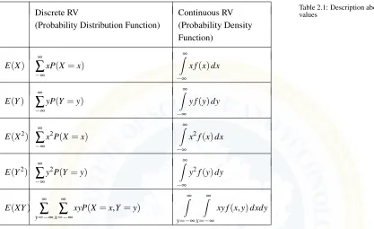
2.2 Problems on Covariance and Correlation

We know that the correlation coefficient is given byρ_XY =Cov(X,Y)

σ_Xσ_Y whereCov(X,Y) =E(XY)−E(X)E(Y), σX =

E(X2)−[E(X)]2andσY =E(Y

2₎₋_[_E₍_Y_)]2_{. The expected values for discrete and continuous distributions are described} in the Table 2.1.

Discrete RV Continuous RV

(Probability Distribution Function) (Probability Density Function)

E(X) ∞

∑

−∞

xP(X=x)

∞ Z

−∞

x f(x)dx

E(Y) ∞

∑

−∞

yP(Y=y)

∞ Z

−∞

y f(y)dy

E(X2) ∞

∑

−∞

x2P(X=x)

∞ Z

−∞

x2f(x)dx

E(Y2) ∞

∑

−∞

y2P(Y =y)

∞ Z

−∞

y2f(y)dy

E(XY) ∞

∑

y=−∞ ∞

∑

x=−∞

xyP(X=x,Y =y)

∞ Z y=−∞ ∞ Z x=−∞

xy f(x,y)dxdy

Table 2.1: Description about Expected values

Further the Expected values in the discrete cases are equivalent to the average values. So the following formula may be used to calculate the expected values in discrete case.

E(X) =∑X

n , E(Y) =

∑Y

n , E(X

2_{) =} ∑X2 n , E(Y

2_{) =}∑Y2

n andE(XY) =

∑XY

n

r_XY =r_UV =Cov(X,Y)

σX×σY

σ_X×σ_Y =

E(XY)−E(X)E(Y) q

E(X2₎₋_[_E₍_X_)]2

× q

E(Y2₎₋_[_E₍_Y_)]2

Substituting the corresponding values and simplifying, we get

σ_X×σ_Y =

N∑(uv)−∑(u)×∑(v)

r n

N∑(u2)−(∑(u))2

orn

N∑(v2)−(∑(v))2

o

whereu=X−Aor X−A

h ,v=Y−Bor Y−B

(23)

Example 2.2.1 Find the correlation co-efficient for the following data:

X 27 28 29 30 32 32 33

Y 17 18 19 19 21 20 21 .

Solution: Karl Pearson’s correlation coefficient is given by

rXY =rUV =

N∑(uv)−∑(u)×∑(v)

r n

N∑(u2)−(∑(u))2

orn

N∑(v2)−(∑(v))2

o

withu=X−30 andv=Y−19

X Y u=X−30 v=Y−19 u2 v2 uv

27 17 -3 -2 9 4 6

28 18 -2 -1 4 1 2

29 19 -1 0 1 0 0

30 19 0 0 0 0 0

32 21 2 2 4 4 4

32 20 2 1 4 1 2

33 21 3 2 9 4 6

211 135 1 2 31 14 20

Now,

rXY =rUV =

N∑(uv)−∑(u)×∑(v)

r n

N∑(u2)−(∑(u))2

orn

N∑(v2)−(∑(v))2

o

= _p 7×20−1×2

{7×31−1}p

{7×14−4}

= √ 138

216√94= 138

142.49=0.968.

Example 2.2.2 Find the correlation co-efficient for the following data:

X 62 64 65 69 70 71 72 74

Y 126 125 139 145 165 152 180 208 .

Solution: Karl Pearson’s correlation coefficient is given by

rXY =rUV =

N∑(uv)−∑(u)×∑(v)

r n

N∑(u2)−(∑(u))2

orn

N∑(v2)−(∑(v))2

o

withu=X−69 andv=Y−152

(24)

X Y u=X−69 v=Y−152 u2 v2 uv

62 126 -7 -26 49 676 182

64 125 -5 -27 25 729 135

65 139 -4 -13 16 169 52

69 145 0 -7 0 49 0

70 165 1 13 1 169 13

71 152 2 0 4 0 0

72 180 3 28 9 784 84

74 208 5 56 25 3136 280

-5 24 129 5712 746

Now,

rXY =rUV =

N∑(uv)−∑(u)×∑(v)

r n

N∑(u2)−(∑(u))2

orn

N∑(v2)−(∑(v))2

o

= p 8×746−(−5)×24

{8×129−25}p{8×5712−(24)2_}

= _p 5968+120

{1032−25}p

{45696−576}

= √ 6088

1007√45120=

6088

31.733×212.415=0.903.

Example 2.2.3 Calculate the covariance and Pearson’s correlation co-efficient for the following data:

Marksy Agex

16−17 17−18 18−19 19−20

30−40 20 10 3 2

40−50 4 28 6 4

50−60 − 5 11 −

60−70 − − 2 −

70−80 − − − 5

.

Hints/Solution:

Let us take the assumed mean inxasA=18.5 and inyasB=55 withh=1 andk=10.

Now letX=x−A h =

x−18.5

1 andY =

y−B k =

y−55

10 with following assumptions.

(25)

Y

X

16.5 17.5 18.5 19.5 fy Y Y fy Y2fy XY fxy

fxy=20 10 3 2 35 −2 −70 140

35 XY=4 2 0 −4

XY fxy=80 20 0 −2 96

fxy=4 28 6 4 42 −1 −42 42

45 XY=2 1 0 −1

XY fxy=8 28 0 −4 32

fxy=0 5 11 0 16 0 0 0

55 XY=0 0 0 0

XY fxy=0 0 0 0 0

fxy=0 0 2 0 2 1 2 2

65 XY=−2 −1 0 1

XY fxy=0 0 0 0 0

fxy=0 0 0 5 5 2 10 20

75 XY=−4 −2 0 2

XY fxy=0 0 0 10 10

fx 24 43 22 11 N=100 0 −100 204 138

X −2 −1 0 1 −2

X fx −48 −43 0 11 −80

X2fx 96 43 0 11 150

XY fxy 88 48 0 2 138

.

Here

rxy=rXY =

N∑(fXYXY)−∑(fXX)×∑(fYY) r

n

N∑(fXX

2

)−(∑(fXX))

2o n

N∑(fYY

2

)−(∑(fYY))

2o

rxy=rXY =

100(138)−(−80)(−100)

r n

100(150)−(−80)2o n100(204)−(−100)2o

rxy=rXY =

58

p

{86} {104}=0.613

withN=

_∑

fx=

∑

fy=100

From the above calculations we find that

Covariance ofXandY isCov(X,Y) =0.58, SD ofXisσ_X =

√

0.86=0.927 and SD ofY isσ_Y =

√

1.04=1.019

(26)

IV

2.1 Two Dimensional Discrete and Continuous Distributions

Unit-2-Two Dimensional Random

(27)

2.0.1

(28)

Two Dimensional Random Variables-Session 10 and 11

2.1 Two Dimensional Discrete and Continuous Distributions

2.1 Transformation of random variables

We will now look at what happens when we apply a function to random variables. We first look at the simple case where there is just one variable, and then move on to the general case where we have multiple variables and can mix them together.

Single random variable

Theorem 2.1.1 IfXis a continuous random variable with a pdf f(x), andh(x)is a continuous, strictly increasing func-tion withh−1(x)differentiable, thenY =h(X)is a random variable with pdf

fY(y) = fX(h−1(y)) d dyh

−1₍_y₎_.

Proof.

FY(y) =P(Y ≤y)

=P(h(X)≤y) =P(X≤h−1(y)) =F(h−1(y))

Take the derivative with respect toyto obtain

fY(y) =FY0(y) = f(h −1

(y)) d

dyh −1

(29)

2.1.3 - 2.1. TWODIMENSIONALDISCRETE ANDCONTINUOUSDISTRIBUTIONS

It is often easier to redo the proof than to remember the result.

Description 2.1.1 LetX∼U[0, 1]. LetY =−logX. Then

P(Y ≤y) =P(−logX≤y) =P(X≥e−y) =1−e−y.

But this is the cumulative distribution function ofE(1). SoY is exponentially distributed withλ=1.

In general, we get the following result:

Theorem 2.1.2 LetU∼U[0, 1]. For any strictly increasing distribution functionF, the random variableX=F−1Uhas distribution functionF.

Proof.

P(X≤x) =P(F−1(U)≤x) =P(U≤F(x)) =F(x).

This condition “strictly increasing” is needed for the inverse to exist. If it is not, we can define

F−1(u) =inf{x:F(x)≥u, 0<u<1},

and the same result holds.

This can also be done for discrete random variablesP(X=xi) =piby letting

X=xjif j−1

∑

i=0

pi≤U< j

∑

i=0

pi,

forU∼U[0, 1].

Multiple random variables

SupposeX1,X2,· · ·,Xnare random variables with joint pdf f. Let

Y1=r1(X1,· · ·,Xn)

Y2=r2(X1,· · ·,Xn) ..

.

Yn=rn(X1,· · ·,Xn).

For example, we might haveY1= X1 X1+X2

andY2=X1+X2.

LetR⊆Rn_{such that}_P₍₍_X

1,· · ·,Xn)∈R) =1, i.e.Ris the set of all values(Xi)can take.

(30)

SupposeSis the image ofRunder the above transformation, and the mapR→Sis bijective. Then there exists an inverse function

X1=s1(Y1,· · ·,Yn)

X2=s2(Y1,· · ·,Yn) ..

.

Xn=sn(Y1,· · ·,Yn).

For example, ifX1,X2refers to the coordinates of a random point in Cartesian coordinates,Y1,Y2might be the coordi-nates in polar coordicoordi-nates.

Definition 2.1.1 — Jacobian determinant. Suppose ∂si ∂yj

exists and is continuous at every point(y1,· · ·,yn)∈S. Then theJacobian determinantis

J= ∂(s1,· · ·,sn)

∂(y1,· · ·,yn)

=det       

∂s1

∂y1

· · · ∂s1

∂yn ..

. . .. ...

∂sn ∂y1

· · · ∂sn

∂yn       

TakeA⊆RandB=r(A). Then using results from IA Vector Calculus, we get

P((X1,· · ·,Xn)∈A) = Z

A

f(x1,· · ·,xn)dx1· · ·dxn

= Z

B

f(s1(y1,· · ·yn),s2,· · ·,sn)|J|dy1· · ·dyn

=P((Y1,· · ·Yn)∈B). So

Proposition 2.1.1 (Y1,· · ·,Yn)has density

g(y1,· · ·,yn) = f(s1(y1,· · ·,yn),· · ·sn(y1,· · ·,yn))|J|

if(y1,· · ·,yn)∈S, 0 otherwise.

Description 2.1.2 Suppose(X,Y)has density

f(x,y) =  



4xy 0≤x≤1, 0≤y≤1 0 otherwise

We see thatXandY are independent, with each having a density f(x) =2x.

DefineU=X/Y,V =XY. Then we haveX=√UVandY =pV/U.

The Jacobian is

det ∂x/∂u ∂x/∂v ∂y/∂u ∂y/∂v

! =det    1 2 p

v/u 1

2 p

u/v

−1 2

p

v/u3 1 2

p 1/uv



 =

(31)

Alternatively, we can find this by considering

det ∂u/∂x ∂u/∂y ∂v/∂x ∂u/∂y !

=2u,

and then inverting the matrix. So

g(u,v) =4√uv r

v u

1 2u =

2v u ,

if(u,v)is in the imageS, 0 otherwise. So

g(u,v) =2v

uI[(u,v)∈S].

Since this is not separable, we know thatUandV are not independent.

In the linear case, life is easy. Suppose

Y=     Y1 .. . Yn     =A     X1 .. . Xn    

=AX

ThenX=A−1Y. Then ∂xi ∂yj

= (A−1)i j. So|J|=|det(A−1)|=|detA|−1. So

g(y1,· · ·,yn) = 1 |detA|f(A

−1_y ).

Description 2.1.3 SupposeX1,X2have joint pdf f(x1,x2). Suppose we want to find the pdf ofY =X1+X2. We let Z=X2. ThenX1=Y−ZandX2=Z. Then

Y Z

!

= 1 1

0 1

! X1 X2 !

=AX

Then|J|=1/|detA|=1. Then

g(y,z) =f(y−z,z)

So

gY(y) = Z ∞

−∞

f(y−z,z)dz= Z ∞

−∞

f(z,y−z)dz.

IfX1andX2are independent,f(x1,x2) = f1(x1)f2(x2). Then

g(y) = Z ∞

−∞f1(z)f2(y−z)dz.

Non-injective transformations

We previously discussed transformation of random variables by injective maps. What if the mapping is not? There is no simple formula for that, and we have to work out each case individually.

(32)

Description 2.1.4 SupposeX has pdff. What is the pdf ofY=|X|?

We use our definition. We have

P(|X| ∈x(a,b)) = Z b

a

f(x) + Z −a

−b

f(x)dx= Z b

a

(f(x) +f(−x))dx.

So

fY(x) =f(x) +f(−x),

which makes sense, since getting|X|=xis equivalent to gettingX=xorX=−x.

Description 2.1.5 SupposeX1∼E(λ),X2∼E(µ)are independent random variables. LetY =min(X1,X2). Then

P(Y≥t) =P(X1≥t,X2≥t) =P(X1≥t)P(X2≥t) =e−λte−µt

=e−(λ+µ)t.

SoY∼E(λ+µ).

Given random variables, not only can we ask for the minimum of the variables, but also ask for, say, the second-smallest one. In general, we define theorder statisticsas follows:

Definition 2.1.2 — Order statistics. Suppose thatX1,· · ·,Xnare some random variables, andY1,· · ·,YnisX1,· · ·,Xnarranged in increasing order, i.e.Y1≤Y2≤ · · · ≤Yn. This is theorder statistics.

We sometimes writeYi=X(i).

Assume theXiare iid with cdfFand pdf f. Then the cdf ofYnis

P(Yn≤y) =P(X1≤y,· · ·,Xn≤y) =P(X1≤y)· · ·P(Xn≤y) =F(y)n. So the pdf ofYnis

d dyF(y)

n₌_{n f}₍_y₎_F₍_y₎n−1_.

Also,

P(Y1≥y) =P(X1≥y,· · ·,Xn≥y) = (1−F(y))n. What about the joint distribution ofY1,Yn?

G(y1,yn) =P(Y1≤y1,Yn≤yn)

=P(Yn≤yn)−P(Y1≥y1,Yn≤yn)

=F(yn)n−(F(yn)−F(y1))n.

Then the pdf is

∂2

∂y1∂yn

G(y1,yn) =n(n−1)(F(yn)−F(y1))n−2f(y1)f(yn).

(33)

Suppose thatδ is sufficiently small that all othern−2Xi’s are very unlikely to fall into[y1,y1+δ)and(yn−δ,yn]. Then to find the probability required, we can treat the sample space as three bins. We want exactly oneXito fall into the

first and last bins, andn−2Xi’s to fall into the middle one. There are _n

1,n−2, 1

=n(n−1)ways of doing so.

The probability of each thing falling into the middle bin isF(yn)−F(y1), and the probabilities of falling into the first and last bins are f(y1)δ andf(yn)δ. Then the probability ofY1∈[y1,y1+δ)andYn∈(yn−δ,yn]is

n(n−1)(F(yn)−F(y1))n−2f(y1)f(yn)δ2,

and the result follows.

We can also find the joint distribution of the order statistics, sayg, since it is just given by

g(y1,· · ·yn) =n!f(y1)· · ·f(yn),

ify1≤y2≤ · · · ≤yn, 0 otherwise. We have this formula because there aren!combinations ofx1,· · ·,xnthat produces a given order statisticsy1,· · ·,yn, and the pdf of each combination is f(y1)· · ·f(yn).

In the case of iid exponential variables, we find a nice distribution for the order statistic.

Description 2.1.6 LetX1,· · ·,Xnbe iidE(λ), andY1,· · ·,Ynbe the order statistic. Let

Z1=Y1

Z2=Y2−Y1 ..

.

Zn=Yn−Yn−1.

These are the distances between the occurrences. We can write this as aZ=AY, with

A=      

1 0 0 · · · 0 −1 1 0 · · · 0

..

. ... ... . .. ... 0 0 0 · · · 1

     

Then det(A) =1 and hence|J|=1. Suppose that the pdf ofZ1,· · ·,Znis, sayh. Then

h(z1,· · ·,zn) =g(y1,· · ·,yn)·1

=n!f(y1)· · ·f(yn)

=n!λne−λ(y1+···+yn)

=n!λne−λ(nz1+(n−1)z2+···+zn)

=

n

∏

i=1

(λi)e−(λi)zn+1−i

Sincehis expressed as a product ofndensity functions, we have

Zi∼E((n+1−i)λ).

with allZiindependent.

(34)

2.2.8 - 2.2. PROBLEMS BASED ONTRANSFORMATION OFRANDOMVARIABLES

2.2 Problems based on Transformation of Random Variables

Example 2.2.1 Given the joint pdf of(X,Y)as f(x,y) =x+y, 0≤x,y≤1, find the pdf ofU=XY.

Hints/Solution:

GivenU=XY and letV =Y.

Transformation equations areu=xyandv=y =⇒ x=u v,y=v.

J= ∂x ∂u ∂x ∂v ∂y ∂u ∂y ∂v = 1 v −u v2 0 1 = 1 v.

f(u,v) =|J|f(x,y) = 1 v

u v+v

, 0≤u≤v, 0≤v≤1.

fU(u) = 1 Z u 1 v u

v+v

dv=2(1−u), 0<u<1

Example 2.2.2 IfXandYare independent exponential random variables with parameters 2 and 3 respectively. Find the density function ofU=X−Y.

Hints/Solution:

Given fX(x) =2e−2x,x≥0 and fY(y) =3e−3x,y≥0.

SinceXandY are independent fX(x)·fY(y) = f(x,y) =6e−(2x+3y). LetU=X−Y andV =Y.

Transformation equations areu=x−yandv=y =⇒ x=u+v,y=v.

J= ∂x ∂u ∂x ∂v ∂y ∂u ∂y ∂v = 1 0 1 1 =1.

f(u,v) =|J|f(x,y) =6e−(2u+3v), v≥ −u,v≥0.

fU(u) = ∞ Z

−u

6e−(2u+3v)dv= 6

5e 3u_,_u_<₀

andfU(u) = ∞ Z

0

6e−(2u+3v)dv=6

5e

(35)

2.3.9 - 2.3. EXERCISE/PRACTICE/ASSIGNMENTPROBLEMS

2.3 Exercise/Practice/Assignment Problems

1. Find the Pearson’s and Spearman’s Correlation Co-efficient and two lines of regression for the following data:

Marks in Statistics MarksinMathematics

47 52 57 62 67

57 3 4 2 − −

62 4 8 8 2 −

67 − 7 12 4 4

72 − 3 10 8 5

77 − − 3 5 8

.

Hint: Use the Formula

rXY =rUV =

N∑(fXYuv)−∑(fXu)×∑(fYv)

r n

N∑(fXu2)−(∑(fXu))2

o n

N∑(fYv2)−(∑(fYv))2

o

withu=X−20 andv=Y−35 orY−35 10

Ans:rXY =0.63

2. Find the Pearson’s and Spearman’s Correlation Co-efficient and two lines of regression for the following data:

MarksY AgeX

18 19 20 21 Total

10−20 4 2 2 − 8

20−30 5 4 6 4 19

30−40 6 8 10 11 35

40−50 4 4 6 8 22

50−60 − 2 4 4 10

60−70 − 2 3 1 6

Total 19 22 31 28 100 .

Ans:rXY =0.1897

3. Calculate the Pearson’s correlation co-efficient and regression equations for the following data:

MarksY AgeX

16−17 17−18 18−19 19−20

30−40 20 10 3 2

40−50 4 28 6 4

50−60 − 5 11 −

60−70 − − 2 −

70−80 − − − 5

.

4. The joint probability distribution of the random variables X and Y are given below:

Y

1 2 3 4 5 6

0 0 0 2k 4k 4k 6k

X 1 4k 4k 8k 8k 8k 8k

2 2k 2k k k 0 2k

Find

(36)

(a) Value of k

(b) Marginal distributions of X and Y (c) P(X≤1)

(d) P(X≤1/Y =2)

(e) P(X<3/Y ≤4)

5. The joint probability function of a two dimensional random variable(X,Y)isf(x,y) =  



c(2x+y), x=0, 1, 2,y=0, 1, 2

0, otherwise

Find

(a) the value ofc

(b) P(X≥1,Y ≥1)

(c) P(X+Y≥1)



c(x+y), x=1, 2, 3,y=1, 2

0, otherwise

Find

(a) the value ofc

(b) P(X≥1,Y ≥1)

(c) P(X+Y≤3)



kxye−12(x2+y2)_, _x_>_0,_y_>₀

0, otherwise

Find

(a) the value ofk

(b) the marginal pdf’s ofXandY

(c) the conditional distribution ofY givenX=x

(d) the conditional distribution ofX givenY =y

(e) P(X≥1/Y ≤1)

(f) P(X+Y≥1)

(g) AreXandY ar independent?



k(x3y+xy3), 0≤x≤2, 0≤y≤2 0, otherwise

Find

(a) the value ofk

(e) P(X≥1

2/Y≤1) (f) P(X+Y≤1)

 x2

8 +xy

2_, ₀_≤_x_≤_{2, 0}_≤_y_≤₁

0, otherwise

Find

(37)

(e) P(X≥1

2/Y≤1) (f) P(X+Y≤1)

(g) P(X>1),P(Y <1

2),P(X>1/Y < 1

2),P(Y < 1

2/X>1),P(X<Y)

10. Given the joint pdf of(X,Y)as f(x,y) =  



4xye−(x2+y2), x,y≥0,

0, otherwise

. Find the pdf ofU=pX2₊_Y2_.

 1 2xe

−y_, ₀_<_x_<_2,_y_>_0,

0, otherwise

. Find the pdf ofU=X+Y.



x+y, 0<x,y<1,

0, otherwise

. Find the pdf ofU=XY.



4xy, 0<x,y<1,

0, otherwise

. Find the joint pdf ofX2andXY.

14. IfXandY are independent random variables follows exponential distributions with unit mean (i.e.meanλ=1 for

both). Find the pdf’s of bothU= X

X+Y andV =X+Y. Are they independent?



2, 0<x<y<1,

0, otherwise

. Find the pdf ofU= X Y.

16. IfX1,X2,. . .,Xnbe independent Poisson variables with parameterλ =2. Use Central Limit Theorem (CLT) to estimateP(120<Sn<160), whereSn=X1+X2+· · ·+Xnandn=75.

17. A random sample of size 100 is taken from a population whose mean is 60 and variance 400. Using CLT to find, with what probability can we assert that the mean of the sample will not differ fromµ=60 by more than 4? 18. A distribution with unknown meanµhas variance 1.5. Use CLT to find how large a sample should be taken from

the distribution in order that the probability will be at least 0.95 that the sample mean will be within 0.5 of the population mean.

19. The life time of a certain brand of tube light may be considered as a random variable with mean 1200 hours and S.D. 250 hours. Find the probability using CLT that the average life time of 60 lights exceeds 1250 hours.

20. A fair coin is tossed 250 times. Find the probability that heads will appear between 120 and 140 times using CLT.

Figure 2.1: Values ofe−λ_.

Contact: (+91) 979 111 666 3 (or)athithas@srmist.edu.in

Visit: https://sites.google.com/site/lecturenotesofathithans/home

(38)

18MAB203T-U2-Book.pdf

18MAB203T-Probability and Stochastic Process

As per 2018 Regulations of SRM

S. ATHITHAN

DEPARTMENT OF MATHEMATICS

FACULTY OF ENGINEERING AND TECHNOLOGY

SRM Institute of Science and Technology,

KATTANKULATHUR-603203

Contents

I

Unit-2-Two Dimensional Random Variables

II

Unit-2-Two Dimensional Random Variables

III

Unit-2-Two Dimensional Random Variables

IV

Unit-2-Two Dimensional Random Variables

Two Dimensional Random Variables-Session 1 and 2

∏

∏

∑

∑

II

-Two Dimensional Random Variables-Session 3 and 5

III

Two Dimensional Random Variables-Session 6,7 and 9

∏

∏

∑

∑

∑

∑

∑

∑

∑

∑

∑

∑

IV

Unit-2-Two Dimensional Random

Two Dimensional Random Variables-Session 10 and 11

∑

∑

∏

_∏

_∑

_∏

_∑

_∑