infocom-ces-scal.pdf

(1)

On the Scalability of Ad Hoc Routing Protocols

C&r A. Santiv8fiez

Bruce McDonald

Ioannis Stavrakakis

Ram Ramanathan

Internet. Research Dept. Elec. & Comp. Eng. Dept. Dept. of Informatics Internet. Research Dept.

BBN Technologies

Northeastern University

University of Athens

BBN Technologies

Cambridge, MA

Boston, MA

Athens, Greece

Cambridge, MA

ramanath @ bbn.com

Ah~rrct-A novel framework is presented for the study of scalability in ad hoc networks. Using this framework, the first asymptotic analysis is provided with respect to network size, mobility, and traffic for each fundamental class of ad hoc routing algorithms. Protocols studied include the fnl- lowing: Plain Flooding (PF), Standard Link State (SLS), Dynamic Source Routing (DSR), Hierarchical Link State (HierLS), Zone Routing Protocol (ZRP), and Hazy Sighted Link State (HSLS). It is shown that PF and ZRP scale better with mobility, SLS and ZRP scale better with respect to traffic, and HSLS scales better with respect to network size. The analysis provides deeper understanding of the limits and trade-offs inherent in mobile ad hoc network routing. Our analysis is complemented with a simulation experiment comparing HSLS and HierLS. An important contribution of this paper is that HSLS is an scalable, easy-to-implement, alternative to hierarchical approaches for large ad hoc networks.

1. INTRODUCTION

Routing protocols for ad hoc networks have been the sub- ject of extensive research over the past several years. Recently, practical applications such as intelligent sensor networks have focused attention on understanding the issues and tradeoffs in network scalability. An important question that arises is : which routing protocol scales the best? The typical answer is: it depends. Unfortunately, the networking community lacks a tenet for understanding the fundamental properties and limitations of ad hoc networks. Hence, a fundamental understanding of what scalability depends on, and how is currently lacking.

One reason for this shortcoming is a lack of sufficient research aimed at general principles and analytical modeling. Scalabil- ity and other performance aspects of ad hoc routing have been studied predominantly via simulations (e.g. [ 11, 121, [ 31) versus theoretical analyses. Simulation results, although extremely useful, are often limited in scope to specific scenarios. Thus, they often fail to produce results that provide the depth of understanding of the limitations of the protocols and their dependence on system parameters and environmental factors desired by researchers. The lack of much needed theoretical analysis in this area is due, we believe, in part to the lack of a common platform to base theoretical comparisons on, and in part due to the abstruse nature of the problem.

This paper focuses on the development of principles and methodologies for the analysis and design of scalable routing strategies for ad hoc networks. Analytical models are developed and results are presented that provide significant insight into the aforementioned dependency and the general performance characteristics of the most important classes of ad hoc network routing algorithms. The theoretical models developed establish the basis for an unbiased analysis and comparison of the relative scalability of several proposed routing protocols.

The first precise (asymptotic) expressions reflecting the im-

pact of network size, traffic intensity and mobility on protocol performance are developed in this paper. Analytical results are presented for a representative set of state-of-the-art protocols in the literature, including : no routing ~ Plain Flooding (PF), proactive ~ Standard Link State (SLS), reactive ~ Dy- namic Source Routing (DSR) 171, hybrid ~ Zone Routing Pro- tocol (ZRP) [ 91, hierarchical ~ Hierarchical Link State (HierLS) [ 81, and limited disemination ~ Hazy Sighted Link State (HSLS) [ 111, techniques. As such, the results provide researchers with improved understanding of the limits and trade-offs inherent in ad hoc network routing. A significant result is that, under the assumptions of this work, HSLS-while being easier to implement ~ scales better than HierLS and ZRP with respect to network size. This analytical result is validated with simulation analysis comparing HSLS and HierLS. Thus, another important contribution of this work is to show that HSLS is an scalable, more efficient alternative than hierarchical approaches for routing in large ad hoc networks. ’

Despite limited prior related theoretical work, there have been notable exceptions. In [ 41 analytical and simulation results are integrated in a study that provides valuable insight into comparative protocol performance. However, it fails to deliver a final analytical result, deferring instead to simulation. Thus, it is dif- ficult to fully understand the interactions among system parameters. The present work closes this gap and provides an understanding of the dynamic interaction among network parameters. The asymptotic capacity of a fixed wireless network was studied in [ 5 1; however, it did not include routing overhead. In con- trast, we,fOCLLs on total overhead (defined later), which includes routing overhead. The impact of mobility on network capacity was studied in 161. They showed that given no restriction on memory size and arbitrarily long delays, mobility increases network capacity. This research, however, focuses on practical scenarios, wherein, delay cannot grow arbitrarily large and mobility reduces the network capacity (degrading performance).

The remainder of this paper is organized as follows: In Section-II we characterize the (total overhead) metric and the network model used. Sections-III - VIII present analysis of the asymptotic performance of PF, SLS, DSR, HierLS, ZRP, and HSLS respectively. Comparison of protocol performance is discussed in Section-IX, focusing on HierLS and HSLS under large network size and including simulation results. Finally, conclusions are presented in Section-X

(2)

11. MODELING PRELIMINARIES

Ths section presents the model assumptions and definitions employed in our analysis.

A. Network model

The following notation will be utilized in this paper: Let N be the number of nodes in the network, d be the average in-degree, L be the average path length (in hops) over all source destination pairs, XI, be the expected number of link status changes that a node detects per second, Xt be the average traffic rate that a node generates in a second (in bps), X, be the average number of new sessions generated by a node per second, and data be the average data packet size (in bits). This work uses the same set of assumptions, based on geographical reasoning, that were presented and discussed in [ 111, [ 121, [ 141, [ 1.51, which are reproduced below for the sake of clarity. 2

. a. 1. As the network size increases, the average in-degree d remains constant.

. a.2. Let A be the area covered by the N nodes of the network, and CJ = N/A be the network average density. Then, the expected (average) number of nodes inside an area Al is approximately CJ Al.

. a.3. The number of nodes that are at distance of Ic or less hops away from a source node increases (on average) as O(d Jc”). The number of nodes exactly k hops away increases as O(d Ic). . a.4. The maximum and average paths (in hops) among nodes in a connected subset of n nodes both increase as O(6). In particular, the maximum path length across the entire network and the average path length across the network (L) increase as O(JN).

. a.5. The traffic that a node generates each second (X, and X,), is independent of the network size N (number of destinations). As the network size increases, the total amount of data transmitted/received by a single node remains constant, but the number of destinations increases (traffic diversity will increase). . a.6. For a given source node, all possible destinations (N - 1 nodes) are equiprobable. The traffic from one node to a given destination decreases as @(l/N).

. a.7. Link status changes are due to mobility. Xl, is directly proportional to the relative node speed.

. a.8. Mobility models : time scaling. Let go/r (2, y) be the probability distribution function of a node position at time 0 second, given that it is known that the node position at time 1 will be (0,O). Then, the probability distribution function of a node position at time t < tl given that the node will be at the position (xtl, yt,) at time tl, is given by gtlt, (2, y, xtl, yt,) =

Assumptions a.1 1 a.8 represents a well-defined network model, still general enough to include most of the typical networking scenarios. The reader is referred to [ 111, and [ 121 for a discussion on these assumptions.

It should be noted that in the case any of the above assumptions does not hold for a particular class of networks, alternative

2Standzd aymptotlc notattlon 15 employed. A function f(n) = O(g(n)) ~\nndarly, f(n) = O(g(n))l d th ere exl\t\ constant\ cl and no [wndarly, c2 and nzl \uch that clg(n) 5 f(n) [\lmdarly f(n) 5 czg(n)l for all n > nl [\lmdarly, n > nz]. Al\o, f(n) = @(g(n)) If and only d f(n) = n(g(n)), and f(n) = O(g(n)).

expressions may be derived by following the same methodology set forth in this paper.

B. Definitions: Total Overhead and Scalability B. 1 Total Overhead

Traditionally, the term overhead has been used in relation to the control overhead, that is, the amount of bandwidth required to construct and maintain a route. However, as shown in [ 111, a protocol’s control overhead alone is not sufficient for assess- ing system performance, as it fails to account for the impact of sub-optimal routes. What is needed is a single metric that is able to capture the routing protocol impact on network performance. For bandwidth-constrained systems, the total overhead introduced in [ 111 and discussed below represents such a metric. First, the minimum tmjfic load of the network must be defined, as follows:

Definition 1: The minimum traffic load

of

a network, is the minimum amount

of

bandwidth required to,forward packets over the shortest distance (in number

of

hops) paths available, assuming all the nodes have instantaneous a priori ,full topology iflformation.

The above definition is independent of the routing protocol being employed, since it does not include the control overhead but assumes that all the nodes are provided a priori global information. It should be noted that it is possible that in fixed networks a node is provided with static optimal routes, and therefore there is no bandwidth consumption above the mini-

rn~m trqjfic load. On the other hand, in mobile scenarios this

is hardly possible. Due to the unpredictability of the movement patterns and the topology they induce, even if static routes are provided so that no control packets are needed, it is extremely unlikely that the static routes so forced remain being the optimal ones during the entire network lifetime. Thus, since sub-optimal routes are present, the actual network bandwidth usage would be greater that the minimum tmjfic load value. This motivates the following definition of a routing protocol total overhead.

Definition 2: The total overhead induced by a routing protocol is the d@erence between the total amount of bandwidth ac- tually consumed by the network running such routing protocol minus the minimum traffic load that would have been required should the nodes had a priori,fLLll topology information.

Thus, the actual bandwidth consumption in a network will be the sum of a protocol independent term, the minimum tmjfic load, and a protocol dependent one, the total overhead. Effec- tive routing protocols should try to reduce the second term (total overhead) as much as possible.

The different sources of overhead that contribute to the total overhead may be grouped and expressed in terms of reactive, proactive, and sub-optimal routing overheads. All of these sources of overhead has been considered in the past, but the total overhead represents the first metric that successfully combines all of them in a unified framework, allowing a tractable model to be derived.

(3)

overhead is a function of the rate of generation of new flows. In dynamic (mobile) networks, however, paths are (re)built not only due to new flows but also due to link failures in an already active path. Thus, in general, the reactive overhead is a function of both traffic and topology change.

The proactive overhead of a protocol is the amount of bandwidth consumed by the protocol in order to propagate route information hcrfore it is needed. This may take place periodically and/or in response to topological changes.

The sub-optimal routing overhead of a protocol is the difference between the bandwidth consumed when transmitting data from all the sources to their destinations using the routes determined by the specific protocol, and the bandwidth that would have been consumed should the data have followed the shortest available path(s). For example, consider a source that is 3 hops away from its destination. If a protocol chooses to deliver one packet following a Ic (Ic > 3) hop path (maybe because of out- of-date information), then (/G - 3) *pa&et-length bits will need to be added to the sub-optimal routing overhead.

The total overhead provides an unbiased metric for performance comparison that reflects bandwidth consumption. De- spite increasing efficiency at the physical and MAC-layers, bandwidth is likely to remain a limiting factor in terms of scalability, which is a crucial element for successful implementation and deployment of ad hoc networks. The authors recognize that total overhead may not fully characterize all the performance aspects relevant to specific applications. However, it can be used without loss of generality as it is proportional to factors including energy consumption, memory and processing requirements, and, furthermore, delay constraints have been shown to be expressed in terms of an equivalent bandwidth [ 13 1.

B.2 Scalability

This work is aimed at the study of the scalability properties of routing protocols for ad hoc networks. However, currently there is not a clear definition of scalability. Indeed, scalability has a different meaning for different people. Thus, we need to define the exact meaning of this term.

Dgfinition 3: Scalability is the ability

of

a network to support the increase

of

its limiting parameters. 3

Thus, scalability is a property. In order to quantify this property, we use the concept of minimum trqjfic load (definition 1) to define the network scalahilit)l,factor as follows:

Dc$nition 4: Let Tr(Xr , X2, . .) he the minimum traffic load experienced by a network underparameters X1, X2, . . . (e.g. network size, mobility rate, data generation rate, etc.). Then, the network scalability factor

of

such a network, with respect to a parameter Xi ( kxi ) is dclfined to he :

k& def lim l%TT(h,b,...) Xiica log xi

The network scalahilit~~,factor is a number that asymptotically relates the increase in network load to the different network parameters. For the class of mobile ad hoc networks under study

3The limiting /x~uneters of a network are those parameter ~ as for example mobility rate, traffic rate, and network size, etc. ~ whose increase causes the network performance to degrade. On the remainder of this work only limiting parameters will be considered, and therefore the term ‘parameter’ will be used in lieu of the term ‘limiting parameter’.

(assumptions a. 1 - a.8) the minimum tmjfic load Tr(Xt,, Xt, IV) is @(&IV1 5), 4 and therefore kxl, = 0, kx, = 1, and xl!N = 1.5.

The network scalahilit~~,factor may be used to compare the scalability properties of different networks (wireline, mobile ad hoc, etc.), and as a result of such comparisons we can say that one class of networks scales better than the other. However, if our desire is to assess whether a network is scalable (an ad- jective) with respect to a parameter X,, then the network rate dependency on such a parameter must be considered.

Definition 5: The network rate Rnet

of

a network is the maximum number

of

hits that can he simultaneously transmitted in a unit

of

time.

For the network rate (Rnet) computation all successful link layer transmissions must be counted, regardless of whether the link layer recipient is the final network-layer destination or not.

Definition 6: A network is said to he scalable with respect to the parameter Xi

if

and only ifi as the parameter X, increases, the network’s minimum traffic load does not increase,faster than the network rate (Rnet) can support. That is,

if

and only ij?

P.Z - x,+x log xi

For example, it has been proved that in mobile ad hoc networks O(N) successful transmissions can be scheduled simultaneously (see for example 1.51, [ 61). The class of networks under study in this work (i.e. resulting from applying power control techniques) are precisely the class of networks that achieves that maximum network rate. Thus, in order for mobile ad hoc network to be regarded as scalable with respect to network size, we will need XPN < 1. Unfortunately this is not the case, and as a consequence ad hoc networks under assumption a.1 through a.8 are not scalable with respect to network size s. Wireline networks, in the other hand, if fully connected may have XPN = 1, and therefore they are potentially scalable (in the bandwidth sense defined here) with respect to network size. Note however, that this scalability requires the nodes’ degree to grow without bound, which may be prohibitely expensive.

Similarly, since the network rate does not increase with mobility or traffic load, then a network will be scalable w.r.t. mobility and traffic if and only if kxl, = 0 and k~,, = 0, respectively. Thus, the networks under this study are scalable w.r.t. mobility, but are not scalable w.r.t. traffic.

Note that similar conclusions may be drawn for scalability w.r.t. additional parameters as for example network density, transmission range e, etc. that are not being considered in our analysis. For example, as transmission range increases (and assuming a infinite size network with regular density) the spatial

4Each node generate At bit\ per second\, that mu\t be retrammltted (m aver age) L tIma (hop\). Thu\, each node Induce a load of XtL, which after addmg all the node\ result\ m a Tr( Xl,, At, N) = At NL. Smce, by a\\umptlon a.4 L ~5 O(m), the above expre\\lon ~5 obtamed.

(4)

reuse decreases and as a consequence network rate decreases as rapidly as e2. Thus, ke should be lower than -2 for the network to be deemed scalable. Since the minimum tmjfic load will only decrease linearly w.r.t. 6 (paths are shortening), qf = -1, and therefore ad hoc networks are not scalable w.r.t. transmission range. ’

Now, after noticing that mobile ad hoc networks are not seal- able with respect to size and traffic, one may ask the meaning of regarding a routing protocol scalable. The remaining of this subsection will clarify this meaning.

Definition 7: Routing protocol’s scalability is the ability

of

a routing protocol to support the continuous increase

of

the network parameters without degrading network perfbmance.

Thus, from the above definition it is clear that the routing protocol scalability is dependent on the scalability properties of the network the protocol is run over. That is, the network own scalabilty properties provides the reference level as to what to expect of a routing protocol. Obviously, if the overhead induced by a routing protocol grows faster than the network rate but slower than the minimum tmjfic load, the routing protocol is not degrading network performance, which is being determined by the minimum tmjfic load.

To quantify a routing protocol scalabilty, the respective scalability factor is defined, based on the total overhead concept (definition 2) as follows:

Definition 8: Let XOu(Al, Aa, . .) be the total overhead induced by routing protocol X, dependent on parameters Al,&, . . . (e.g. network size, mobility rate, data generation rate, etc.). Then, the Protocol X’s routing protocol scalability factor with respect to a parameter & ( p: ) is defined to be :

’ 4 _Az+m _{log Xi}

The routing protocol scalability ,factor provides a basis for comparison among different routing protocols. Finally, to assess whether a routing protocol is scalable, the following definition is used:

Definition 9: A routing protocol X is said to be scalable with respect to the parameter &

if

and only ifi as the parameter & increases, the total overhead induced by such protocol (XOV) does not increase ,faster than the network’s minimum traffic load. That is,

if

and only ij?

Thus, for the class of network under study, a routing protocol X is scalable with respect to network size if and only if & 5 1.5; it is scalable w.r.t. mobility rate if and only if & 5 0; and it is scalable w.r.t. traffic if and only if pft 5 1.

In the remainder of this paper we will derive asymptotic expressions for the total overhead (and therefore the routing protocol scalabilit~~,factor) induced by a representative set of routing protocols. The methodology to be employed consists of com- puting each of the three components of total overhead, namely proactive, reactive and sub-optimal routing, separatedly and then adding them up. Besides the trivial result that Plain Flood-

6Th15 obwwtmn 15 the nmm rea5on behmd our focwmg on network5 wah power control, where the tran~nu~~~on range 15 kept m hne 50 that the network degree 15 kept bounded.

ing (PF) is the only protocol that is scalable with respect to mo- bilty, and that most protocols are scalable with respect to traffic, the more interesting result that HSLS is scalable with respect to network size is found.

III. PLAINFLOODING

In PF, each packet is (re)transmitted by every node in the network (except the destination). Thus, N - 1 transmissions are required for each data packet, when the optimal value (on average) should have been L. Since there are &N data packets generated each second, the additional bandwidth required for transmission of all these packets is dutu (N - 1 - L)&N bps. Since L = O(m), the PF’s sub-optimal routing- and total- <~ve~headpersecondisequalto@(&(N’-N1 ‘)) = 0(&N’). In consequence pftF = 1, p:r = 0, and pgF = 2.

IV. STANDARDLINKSTATE(SLS)

In SLS, a node sends a Link State Update (LSU) to the entire network each time it detects a link status change. A node also sends periodic, soft-state LSUs every Tp seconds. There is no reactive overhead associated with SLS, and since the paths determined are optimal, there is no sub-optimal routing overhead associated with it either.

In SLS, each node generates a LSU at a rate of & per second, so in average there are N& LSUs being generated at any given second. Each LSU is retransmitted at least once per each node (i.e. N times), inducing an overhead of lsu N bits (where lsu is the size of the LSU packet). Then SLS proactive and total- overhead per second is lsu &N’ bps, that is, @(&N’); and b sLs = 0, pfits = 1, and pgLs = 2.

V. DYNAMICS• URCEROUTING(DSR)

In DSR no proactive information is exchanged. A node (source) reaches a destination by flooding the network with a route request (RREQ) message. When a RREQ message reaches the destination (or a node with a cached route towards the destination) a route reply message is sent back to the source, including the newly found route. The source attaches the new route to the header of all subsequent packets to that destination, and any intermediate node along the route uses this attached information to determine the next hop in the route. The present work focuses on DSR without the route cache option (DSR-noRC). A lower bound for DRS-noRC’s total overhead is derived next.

The DSR-noRC reactive overhead must account for RREQ messages generated by new session requests (at a rate & per second per node) and the RREQ messages generated by failures in links that are part of a path currently in use. If we only consider the RREQ messages generated by new session requests, then a lower bound can be obtained.

Each route request message is flooded to the entire network, resulting in N - 1 retransmissions (only the destination does not need to retransmit this message). Thus, each message induces an overhead of size-of-RREQ(N - 1) bits, and there are &N RREQ messages generated every second due to new session requests. Thus, the DSR-noRC reactive overhead per second is fl&N’).

(5)

required for appending the source-route in each data packet. The number of bits appended in each data packet will be proportional to the length Li of path i. Since this length is not shorter than Lypt (the optimal path length), using Lypt instead of Li will result on a lower bound. The extra bandwidth consumed by a packet delivered using a path i (with at least Lypt

retransmissions) will be at least (loga N)(Lypt)‘, where loga N is the minimum length of a node address. The average extra bandwidth per packet over all paths is E{ (log2 N)(Lypt)‘)} 2

(loga N)E{Ly}~ = (loga N)L’ bits. Thus, for each packet sent from a source to a destination there is an average sub-optimul m&g overhead of at least (loga N)L’ bits. Since At N packets are transmitted per second, the sub-optimal m&g overhead induced over the entire network is at least &N(logZ N)L’ bps. Recalling that L = @(a) (assumption a.4) the DSR-noRC sub-optimal routing overhead per second is found to be 0(&N’ loga N) bps.

Combining the previous results, DSR-noRC total overhead

persecondis0(&N’+&N’loga N). A~so,~~~~~~~~ = 1,

DSR-noRC

cl c PAic <= 1, ’ and &sR-nORc > 2. VI. HIERARCHICALLINKSTATE(HIERLS)

In the m-level HierLS routing, network nodes are regarded as level 1 nodes, and level 0 clusters. Level i nodes are grouped into level i clusters, which become level i + 1 nodes, until the number of highest level nodes is below a threshold and therefore they can be grouped (conceptually) into a single level m. Thus,

the value of m is determined dynamically based on the network size, topology, and threshold values.

Link state information inside a level i cluster is aggregated (limiting the rate of LSU generation) and transmitted only to other level i nodes belonging in the same level i cluster (limiting the scope of the LSU). Thus, a node link change may not be sent outside the level 1 cluster (if they do not cause a significant change to higher levels aggregated information), greatly reducing the proactive overhead.

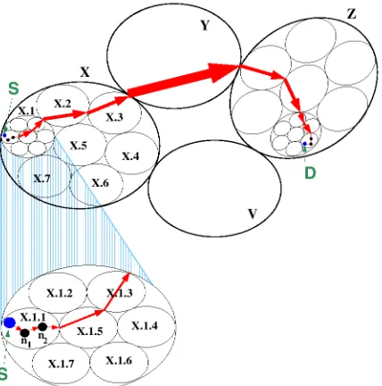
HierLS relies on the Location Management service to inform a source node S of the address of the highest level cluster that contains the desired destination D and does not contain the source node S. For example, consider a 4-level network as shown in Figure 1. S and D are level 1 nodes; X.1.1, X.1.2, etc. are level 2 nodes (level 1 clusters); X.1, X.2, etc. are level 3 nodes (level 2 clusters); X, Y, V, and 2 are level 4 nodes (level 3 clusters); the entire network forms the level 4 cluster. The Location Management (LM) service provides S with the address of the highest level cluster that contains D

and does not contain S (e.g. the level 3 cluster 2 in Figure 1). Node S can then construct a route toward the destination. This route will be formed by a set of links in node S level 1 cluster (X.1.1) a set of level 2 links in node S level 2 clusters (X.1) and so on. In Figure 1 the route found by node S is :

7DSR’s MU/ overhec~d does depend on mobility, since breakages of’ links forming existing routes will trigger route discovery procedures that will induce reactive overhead and/or cause route degradation. Similar to the lower bound derived in this section, an upper bound for DSR’s MU/ overhec~d may be derived by assuming that each link breakage trigger a global route discovery (regardless of’ the link being part of’ an active route or not). Such an upper bound would increase linearly with the mobility rate, and therefore we obtain the upper bound for pfzfRPmoRc <= 1.

Fig. I. A Source (S) Dutmatlon (II) path m HxrLS

S - nl - nz - X.1.5 - X.1.3 - X.2 - X.3 - Y - .Z - D.

When a node outside node S level 1 cluster receives the packet, the node will likely produce the same high-level route towards

D, and will ‘expand’ the high-level links that traverse its cluster using lower level (more detailed) information. In Figure 1 this expansion is shown for the segment .Z - D. The Location Man- agement (LM) service can be implemented in different ways, whether proactive (location update messages), reactive (paging), or hybrid. Typical choices are:

. LMl : Pure reactive. Whenever a node changes its level i clustering membership but remains in the same level i + 1 cluster, this node sends an update to all the nodes inside its level i + 1 cluster. For example, (see Figure 1) if node nz moves inside

cluster X.1.5, i.e. it changes its level 1 cluster membership but does not change its level 2 cluster membership (cluster X.1) then node nz will send a location update to all the nodes inside cluster X.1. The remaining nodes will not be informed.

. LM2: Local paging. In this LM technique, one node in each level 1 cluster assumes the role of a LM server. Also, one node among the level 1 LM servers inside the same level 2 cluster assumes the role of a level 2 LM server, and so on up to level

m. The LM servers form a hierarchical tree. Location updates

are only generated and transmitted between nodes in this tree (LM servers). When a node D changes its level i clustering membership, the LM server of its new level i cluster will send a location update message to the level i + 1 LM server, which in turn will forward the update to all the level i LM servers inside this level i + 1 cluster. Additionally, the level i + 1 LM server checks if the node D is new in the level i + 1 cluster, and if this is the case it will send a location update to its level i + 2 LM server, and so on.

(6)

i - 1 cluster, and so on until all the level 1 LM servers (inside node D’s level i + 1 cluster) are informed of the new level i location information of node D. When a node needs location information about any node in the network, the node pages its level 1 LM server for this information.

. LM3: Global paging. LM3 is similar to LM2. In LM3, however, when a level i LM server receives a location update from a higher level i + 1 LM server, it does not forward this information to the lower level ( i - 1) LM servers. Thus, a lower level (say level j < i) LM server does not have location information for nodes outside its level j cluster. A mechanism for remov- ing outdated location information about nodes that left a level i cluster need to be added to the level i clusters LM servers. Basi- cally, a level 1 LM server that detects that a node left its level 1 cluster will remove the entry corresponding to this node from its own database, and will inform its level 2 LM server. The level 2 LM server will wait for a while for a location update from the new level 1 cluster (if inside the same level 2 cluster) and if no such an update is received it will remove the node entry and will inform its level 3 LM server, and so on until arriving to a LM server that already has information about the new location of the node. When a node needs location information about any node in the network, the node pages its level 1 LM server for the information. If the level 1 LM does not have the required information, it (the level 1 LM server) pages its level 2 LM server, who in turn pages its level 3 LM server, and so on, until a LM server with location information about the desired destination is found.

Approach LMl, the easiest to implement, will induce greater overhead and lower latencies for route establishment. Approach LM2 potentially reduces the bandwidth consumption (for reasonable values of &) but at the expense of complexity (selection and maintenance of LM servers) and an increase in the latency associated with route establishment. However, the asymptotic characteristic of HierLS are identical under LMl and LM2, as will be seen later. Approach LM3 is the more complex to implement. It will induce a significant amount of reactive overhead, but will reduce the amount of overhead induced by mobility. In this paper, results for the HierLS totul overheud for all three LM Techniques are presented in Table I. However, due to space constraints, only the derivation for the total overhead expression for a HierLS-LMl (pure proactive LM technique) will be presented next. The reader is referred to [ 141 or [ 15 1 for the remaining derivations.

A. HierLS-LA41 proactive overhead

A network organized in m level clusters, each of equal size !? (N = P) is considered. Note that !? is predefined while m increases with N.

Under assumption a.7, HierLS-LMl’s proactive asymptotic overhead is dominated by the location management function, that induces an overhead that grows at least as fast as @(.vN’.~) (explained below), where s is the node relative speed. In the other hand, most of the LSUs updates will correspond to level 1 links, and will be propagated inside the level 1 clusters only. thus, LSU packets will induce a proactive overhead that will only grow as fast as & !? N (this is, of course, a lower bound).

HierLS-LMl location management overhead expressions,

can be obtained by considering that the time a node takes to change its level m - 1 cluster is directly proportional to the diameter of this level m - 1 cluster and inversely proportional to

the node’s relative speed s. Since the level m - 1 cluster size is N/k, then the cluster diameter is Q(m) Under approach LMl, the new location information will have to be forwarded to all the nodes inside the level m cluster (the entire network). Thus, every node will send a location update message to the entire network (N transmissions) each @(m/s) seconds, inducing an overhead of @( & sfl) bits every second. Adding up all nodes contributions, the proactive overhead per second due to level m - 1 clusters membership change is @(v%N’ ‘). Regarding the location updates generated due to level m - i

membership change, it can be seen that a level m - i cluster is !F1 times smaller than a level m - 1 cluster, and consequently

a level m-i cluster’s diameter is !?y times smaller than a level

m - 1 cluster’s diameter. Thus, the generation rate of location updates due to level m - i membership changes is !?q times

larger than the rate induced by level m - 1 changes. Also, since

the new location information will have to be transmitted to all the nodes inside the current level m - i + 1 cluster, then the

number of transmissions required for each packet decreases by a factor of &(‘-‘) with respect to the number of transmissions induced by level m - 1 changes, which results in a net reduction

of KY. Then, the overhead due to all location updates is :

Lot-Upd-Cost = @(v%~N~.~)[l + k-; + k-l + . .]

= @(v’%sN~~) ’ 1-m

Thus, the location management overhead is @(&cN1.5) bps (by assumption a.7, & is proportional to s). Combining this value with the lower bound obtained for the LSU-induced overhead (0(&N)), it is concluded that the HierLS-LMl pmxfive overhead is @(&cN1.5).

B. HierLS-LA41 sub-optimal routing overhead

To estimate the sub-optimal routing overhead, it is assumed that each level i (beginning with level 2) increases the actual route length by a factor fZ (fi depends on the value of !?, the LSU triggering thresholds, and is typically close to 1, for example f = 1.05 means a 5% increase in the route length). Thus, if the optimal path length is 1, then the actual path length will be IIizyfi 1. Let f be the geometric average of the set {fi}, that is, f = (IIpafi)A. Then, the sub-optimul routing overhead induced by a packet transmission is dutu [fmP1 - 1] 1 = dutu [k@‘g~ f)(mP1) - 1] 1 = dutu [;’ - 1] 1, where 6 = logk f. There are &N packets generated each second, thus the average sub-optimal routing overhead per second is dutu ($’ - 1) L&N. Since L is e(m), we finally get that the HierLS-LMl sub-optimal routing overhead per second is @(AtN1.5+‘).

C. HierLS-LA41 total overhead

(7)

HivLS-LMl

h = L PAic HivLS-LMl = 1, and ,,;ie~L-Ml =

1.5 + & > 1.5 (HierLS is ulmost scalable w.r.t. netwrok size).

VII. ZONE ROUTING PROTOCOL (ZRP)

ZRP is a hybrid approach, combining a proactive and a reactive part, trying to minimize the sum of their respective overheads. In ZRP, a node disseminates event-driven LSUs to its k- hop neighbors (nodes at a distance, in hops, of !? or less). Thus, each node has full knowledge of its &hop neighborhood and may forward packets to any node within it. When a node needs to forward a packet outside its k-hop neighborhood, it sends a route request to a subset of the nodes in the network, namely the ‘border nodes’. The ‘border nodes’ will have enough information about their &hop neighborhoods to decide whether to reply to the route request or to forward it to its own set of ‘border’ nodes. The route formed will be described in terms of the ‘border’ nodes only, thus allowing ‘border’ nodes to locally recover from individual link failures, reducing the overhead induced by route maintenance procedures.

The following lower bound for ZRP’ total overhead (.ZRP,,V) was obtained:

Due to space limitations, the derivation of the ZRP total overheud was left out of the paper. Once again, the reader is referred to [ 141 or [ 1.5 1 for the complete derivation.

Note that the asymptotic expression provides us with much more information about the parameters interactions than the scalability factors, which are computed assuming that just one parameter is increased while the others remain fixed. For ZRP, b zRp = 0 (pure proactive mode), 0 < pfifp <= 1 (pure reactive mode, similar to DSR’s), and pgRp 2 1.66. Note that the information provided by the ,~~alabilt~~,fa~to~,~ is incomplete, and it hinds the fact that the exponential rates of increase of ZRP’s total overhead with respect to mobility and traffic always add up to at least 1, as can be seen from the total overhead’s asymptotic expressions.

VIII. HAZY SIGHTED LINK STATE (HSLS)

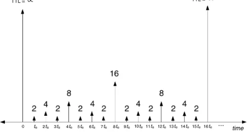
HSLS is based on the observation that nodes that are far away do not need to have complete topological information in order to make a good next hop decision. Thus, propagating every link status change over the entire network may not be necessary. In a highly mobile environment, a node running HSLS will transmit - provided that there is a need to - a LSU only at particular time instants that are multiples of te seconds. Thus, potentially several link changes are ‘collected’ and transmitted every te seconds. The Time Tb Live (TTL) field of the LSU packet is set to a value (which specifies how far the LSU will be propagated) that is a function of the current time index as explained below. After one global LSU transmission ~ LSU that travels over the entire network, i.e. TTL field set to infinity, as for example during initialization ~ a node ‘wakes up’ every te seconds and sends a LSU with TTL set to 2 if there has been a link status change in

16

8 8

t* ... _t/me

Fig. 2. HSLS’s LSU gmemtion process (mobility is high)

the last te seconds. Also, the node wakes up every 2te seconds and transmits a LSU with TTL set to 4 if there has been a link status change in the last 2te seconds. In general, a node wakes up every 2’-‘te (i = 1,2,3, . ..) seconds and transmits a LSU with TTL set to 2% if there has been a link status change in the last 2’-‘tc seconds. If a packet TTL field value (2’) is greater than the distance from this node to any other node in the network (which will cause the LSU to reach the entire network), the TTL field of the LSU is reset to infinity (global LSU), and the algorithm is re-initiated.

Nodes that are at most two hops away from a node, say X, will receive information about node X’s link status change at most after te seconds. Nodes that are more than 2 but at most 4 hops away from X will receive information about any of X links change at most after 2tc seconds. In general, nodes that are more than 2’-’ but at most 2’ hops away from X will receive information about any of X links change at most after 2ip1tc seconds. Figure 2 shows an example of HSLS’s LSU generation process when mobility is high and in consequence LSUs are always generated. An arrow with a number over it indicates that at that time instant a LSU (with TTL field set to the indicated value) was generated and transmitted. Figure 2 assumes that the node executing HSLS computes its distance to the node farthest away to be between 17 and 32 hops, and therefore it replaces the TTL value of 32 with the value infinity, resetting the algorithm at time 16tC. The reader is referred to [ 111 and [ 121 for more details about HSLS.

A. HSLS proactive overhead

A highly mobile environment (i.e. a LSU is generated every time interval) is considered. All the different LSUs (re)transmissions due to LSUs generated by a node, say X, will be added and then averaged over time. The value obtained will be multiplied by the number of nodes in the network to get the pmxtive overhead. LSUs will be grouped based on their TTL value at the time they were generated, beginning with the LSUs with larger TTL values.

(8)

is a time-changing value that is not being timely updated. The above observation, however, will have little impact on the value of Rz, which may be assumed roughly constant over time.

Let’s consider what happens at time Rzte (16& in figure 2). At this time node X sends a LSU to the entire network and the algorithm is re-initiated. Thus, every Rztc seconds node X induces N transmissions, and therefore the bandwidth consumption due to these global LSUs is e, _{Lz e}where lsu is the average length of a LSU packet.

The second larger TTL is Rz, and LSUs with this TTL are generated $$te seconds after a global LSU is sent (times Ste in figure 2). Recalling that the timers are reset at time Rztc, we

notice that the interval between consecutive generation times is

(Rztc - %te) + % te = Rzte. Thus, the generation rate of LSUs with TTL equal to Rz is & (the same as the generation rate of global LSUs). These LSL?; will not reach all the nodes in the network but only a fraction fZ. From assumption a.3, fZ should be around (Rz/MDz)‘, i.e., fZ E [0.25,1]. In practical situations, due to boundary effects (i.e. the number of nodes at a maximum distance MIJZ is small), we obtain that typically fZ is in the interval [0.5,1]. Thus, the bandwidth consumption due to LSUs with TTL equal to Rz is w.

For the remaining TTL values, ‘b&ndary7 conditions are no longer relevant. Thus, for TTL equal to Rz/2 the generation rate doubles (e.g. LSUs with TTL equal to 8 are sent at times 4&, 12&, . . in figure 2) and the number of transmissions induced per LSU is reduced by a factor of 4 (because of assumption a.3, and the fact that the TTL values are reduced to a half); thus the total effect is a reduction by a factor of 2 with respect the bandwidth consumption due to LSUs with TTL equal to Rz. The same argument applies for TTL equal to

Rz/4, Rz/8, . . . . 2, I. ’ Finally, the total bandwidth consumption due to all the LSUs generated by node x is equal to :

Since the size of a LSU depends only on the node density (bounded on average), fZ is bounded below 1, and Rz is @(v%) (assumption a.4); the pmxtive overhead per second induced by one node is 0(c). Since there are N nodes, the

proactive overhead per second induced by the entire network is

O(F).

Due to space constraints, the complete derivation was left out of the paper. Below, an insight into it is provided. The reader is referred to [ 141 or [ 15 1 for the actual derivation.

Let tELap be the maximum time elapsed since ‘fresh’ LSU information about a destination /G hops away was last received. HSLS induces a quasi-linear relationship between tELap and !?. In general, % 5 T 5 te. Thus, the ratio between the time

elapsed since fresh information was received and distance is

bounded by te, independently of network size or distance to the destination. Based on the mobility model assumption a.8 (time scaling), this will cause the probability of a sub-optimal next hop decision to be bounded9, and the fraction of the increase of the sub-optimal routes (with respect to the optimal ones) to also be bounded independently of network size. Then, for a fixed value of te, HSLS sub-optimal routing overhead will increase as C3(AtN1.5).

To investigate the dependence of the sub-optimal routing

overhead on the time te, a more precise mobility model need to be defined. Assuming a mobility model that induces an exponential residence time on a given area, HSLS sub-optimal routing overhead was found to be equal to : @((eAicteK4 - l)&N1.5), where /Q is a constant.

C. HSLS total overhead

There is no reactive overhead associated with HSLS. Thus, the HSLS total overhead for the class of networks analyzed in the previous subsections is equal to :

The value of te should be tuned to optimize performance. For a moment, let’s use the approximation eZ - 1 z Z, where z =

AlcteKd. Thus:

Choosing the value of te that minimizes the above expression we get te = @( &), z = 0(s), and HSLSoV =

@(&&N1.5). The previous expression would define the asymptotic behavior of HSLS’s total overhead only if our approximation eZ - 1 E x is valid. Indeed, if & grows asymptotically faster than &, the value of z goes to zero and the approximation ex - 1 E x is valid. On the other hand, if & grows asymptotically faster than &, the approximation will not be valid. In this case, since the exponential function is the fastest growing, it is desirable to maintain the product Alcte (and therefore the value of p) bounded and therefore we choose te = @( &). Thus, the HSLS totul overheud in this scenario be- comes @(h1,5(& + At)) = @(AL~N’.~), where the last equal- ity holds due to our assumption that & grows asymptotically faster than & and therefore & dominates the previous expression. Thus, the HSLS’s total overhead is :

Also, it can be noted that pEsLs = U.5, pEfLs = 1, and pEsLs = 1.5. Th us, HSLS is the only protocol that is scalable

with respect to network size.

(9)

IX. COMPARATIVE STUDY

In the previous sections the .~~alab~l~t~~,fa~t~~~.~ of several representative routing protocols have been derived. From those results we concluded that PF is the only protocol known to be scalable w.r.t. mobility (p.+ pF = O), while all of the protocols were scalable w.r.t. traffic. More interesting was to find that HSLS is the only protocol scalable with respect to network size (pN HsLs = 1.5). However, much more information about the protocol parameter’s interactions may be derived from the asymptotic total overhead expressions, which are summarized in Table I.

Table I presents our results for the total overhead when the tunable parameters are selected to optimize performance (or at least, optimize the lower bounds derived before). These results increase our understanding of the limits and provide valuable insight about the behavior of several representative routing protocols. The better understanding of these limits will help network designers to better identify the class of protocols to en- gage depending on their operating scenario. For example, if the designer’s main concern is network size, it can be noted that Hi- erLS and HSLS scale better than the others. Similarly, if traffic intensity is the most demanding requirement, then SLS and ZRP are to be preferred since they scale better with respect to traffic (total overhead is independent of At); HSLS follows as it scales as @(a), and PF, DSR, and HierLS are the last since their total overhead increases linearly with traffic. ‘a

Similarly with respect to the rate of topological change, we observe that PF may be preferred (if size and traffic are small and the rate of topological change increases too rapidly), since its total overhead is independent of the rate of topological change. Provably next will be ZRP and DSR since their lower bounds are independent of the rate of topological changes. The bounds are not necessarily tight, and ZRP’s and DSR’s behavior should depend somewhat of the rate of topological change. Fi- nally, for SLS, HierLS, and HSLS we know (as opposed to DSR and ZRP where we suppose) that their total overhead increase linearly with the rate of topological change.

It is interesting to note that when only the traffic or the mobility is increased (but not both), ZRP can achieve almost the best performance in each case. ” However, if mobility and traffic increase at the same rate; that is, & = @(A) and & = @(A) (for some parameter A), then ZRP’s total overhead (0(AN1.66)) will present the same scalability properties as HSLS’s (@(AN1.5)) and HierLS’s (@(AN1.5+‘)) with respect to A, with the difference that ZRP does not scale as well as the other two with respect to size.

These and more complex analyses can be derived from the expression presented in this paper, when different parameters are modified simultaneously accordingly with the scenario the designer is interested in.

loIt is interesting to note that HSLS SC&S better with tmffic intensities than HierLS (the only other protocol that SC&S well with size). This result may have nn intuitive explnnntion in the fact that HierLS never attempts to find optinxd routes towards the destination, even under slowly changing conditions. HSLS on the other hand, may eventnnIly obtain Ml topology information ~ rind therefore optimal routes ~ if’ the rate of’topologicnI changes is small with respect to l/&, as is the case when & grows faster thnn &.

“Almost, because ZRP cnn not achieve the independence of’ MU/ overhec~d from mobility. PF does.

PF 0(&N’) Always

SLS _@C&J? Always

DSR 0(&N’ + AtN2 loga N) no Route Cache HierLS C3(AtcN1.5 + AtN1 5+6) LMl or LM2

@(&Nlog N + &N1 5+h) LM3

ZRP WtcN21 kc = ws/m

O&N’) kc = ~CJwV &j N:) otherwise HSLS C3(&i&N1.5) _{kc = ~~~t~}

@(AL,~N’.~) _{hc = fqh)}

TABLE I ASYMPTOTICTOTALOVERHEADEXPRESSIONS.

HSLS has better asymptotic properties than HierLS, which means that as size increases HSLS eventually outperform Hi- erLS. The idea of HSLS ~ being much more simple to implement ~ outperforming HierLS is counter-intuitive. A first re- action to this result will likely be to assume that the constants involved in the asymptotic analysis may be too large, prevent- ing HSLS from outperform HierLS under ‘reasonable’ scenario. Thus, the authors relied on a couple of simulation experiment to validate if, in effect, HSLS may outperform HierLS even under moderate network size and traffic load.

A. A simulation experiment: HSLS vs. HierLS-LA41

Table II shows the simulation results obtained by OPNET for a 400-node network where nodes are randomly located on a square of area equal to 320 square miles (i.e. density is 1.25 nodes per square mile). Each node choose a random direction among 4 possible values, and move on that direction at 28.8 mph. Upon reaching the area boundaries, a node bounces back. The radio link capacity was 1.676 Mbps. Simulation were run for 3.50 seconds, leaving the first 50 seconds for protocol initialization, and transmitting packets (60 8kbps streams) for the remaining 300 seconds. The HierLS approach simulated was of the type HierLS-LMl, and corresponds to the DAWN project [ 101 modification of the MMWN clustering protocol [ 81. The minimum and maximum cluster size were set to 9 and 35 respectively.

The metric of interest is the throughput (i.e. fraction of packets successfully delivered). The simulation results presented are not a comprehensive study of the relative performance of HierLS versus HSLS under all possible scenarios. They just presents and example of a real-life situation where HSLS outperform HierLS, and complement our theoretical analysis. The theoretical analysis focuses on asymptotically large network, heavy traffic load, and saturation conditions where the remaining capacity determines the protocol performance. The simulation results, in the other hand, refer to medium size networks with moderate loads, where depending on the MAC employed, other factors may have more weight over the protocols performance.

(10)

Protocol UNRELIABLE RELIABLE

HSLS 0.2454 0.7991 _J

HierLS-LMl 0.0668 0.3445 TABLE11

THROUGHPUT OF A 400 NODE NETWORK

CSMA, packets were retransmitted up to 10 times if a MAC- level ACK was not received in a reasonable time. We can see that in both cases HSLS outperforms HierLS, although the relative difference is reduced under the reliable MAC case. This can be explained considering that the high rate of collisions experienced under unreliable CSMA favored shorter paths. For nodes close by, HSLS may provide almost optimal routes while HierLS routes may be far from optimal if the destination belong to a neighboring cluster. Thus, we can see that unreliable MAC biases towards HSLS. Another factor to take into account is the latency to detect link up/downs. Under HierLS this information is synchronized among all the nodes in the cluster and therefore some latency is enforced to avoid flapping. In HSLS, in the other hand, each node may have its own view of the network, and as a consequence a node may be more agressive in tem- porarily turning links down without informing other nodes. As a consequence, HSLS is more agressive and reacts much faster to link degradation, using alternate paths if available.

It can be seen that the previous results are highly influenced for another factors such as the MAC protocol being used, the quality of the links that neighbor discovery declares up, the latency on detecting link failures, etc. So, whether HSLS or Hi- erLS should be preferred for a particular scenario, depends on the particular constraints (for example, if memory or processing time is an issue, HierLS may be preferred since it require to store/process an smaller topology table). The present work, however, provides some guidelines, suggesting that as traffic, network size, and data rate increases, and a better MAC is employed (allowing to achieve the full channel capacity), HSLS should tend to be preferred.

X. CONCLUSIONS

The applications for ad hoc networking are only beginning to be recognized. However, before practical implementations are possible, it is necessary to design scalable systems. Hence, scalability has become a dominant objective of ad hoc network algorithm designers. Unfortunately, the community lacks a basic tenet for understanding the fundamental limitations and invari- ants associated with ad hoc networks.

This paper addresses this shortcoming by presenting a novel and powerful framework (the total overhead criteria) that allows for an analytical comparison, and deeper understanding of the characteristics and tradeoffs associated with various classes of routing protocols for mobile networks. This framework, first introduced in [ 111 to analyze a family of link state protocol vari- ants, was fully developed in this paper and applied to study a variety of protocols that have been proposed and analyzed via simulation methodologies in the literature.

The analytical methods developed in this paper and the result-

ing asymptotic analysis of total overhead provide an important contribution to the field that promises to shed new light on the fundamental limitations and underlying characteristics of mobile networks in general, and in the studied protocols in particular. It was found that, among the protocol studied, PF is the only protocol that scales w.r.t. mobility, all of them scale w.r.t. traffic, and HSLS is the only one that scales w.r.t. network size (note that HierLS almost scale w.r.t. network size). Thus, the results for HSLS ~ a novel, easy-to-implement link state variant ~ showed that the implementation of a complex hierarchy was not mandatory for scalability. A more focused comparison between HierLS and HSLS was undertaken, and as a result, HSLS was established as a competitive alternative to HierLS.

Finally, this work is only a first step. Greater understanding is required of cross-layer interactions and the impact of more general mobility models and traffic workloads. We hope this work will help to lay a foundation for a renewed approach to research into ad hoc networks. The success of this technology depends on rigorous techniques and proof of concepts.

REFERENCES

J. Broth, D. M&z, D. Johnxm, Y. Hu, and J. Jetcheva, “ A PerGxnxmce Compul5on of MultIhop W&e55 Ad Hoc Network Routmg Protocols,” Prweedingy of MOBICOM’98, Dallas, TX., October 19%

V. D. Park, and S. Cor5on, “ A Performance Compul5on of the Temporally Ordered Routmg Algorithm md Ideal Lmk St& Routmg,” Prweedingy of IEEE Swp~~iwn on Cwnputer~ and Cwnmunicchn~ ISCC‘98, Athen5, Greece, June 19%

C. E. PerkIm, E. M. Royer, S. R. D+ md M. K. Muma, “Performmce Compul5on of Two On Demand Routmg Protocol5 for Ad Hoc Net works”, IEEE Perwmd C~mmunichm~ Mgcaine, Vol. X, No. I, Feb. 2001.

P. Jxquet and L. Vxnnot, ‘Overhead m Mobde Ad hoc Network Proto col5”, INRIA Rewurch Report 3965, Inytitut Nutiwml de Recherche en Inf?rmatique et en Aut~matique (INRIAj, Fmnce, June 2000.

P. Gupta and P.R. Kumx “The Capxlty of Wxele55 Networks”, IEEE Trcmwcti~n on Information Thaw], 46 (2):3Xx 404, Mzch 2000. M. Gro55glu5er and D. T5e. “Mobdlty Increa5e5 the Capxlty of Ad hoc Wxele55 Networks”, m Prxceedingy of IEEE Inf~c~m’2001, Anchorage, Alaska, Aprd 200 I.

D. B. Johmon md D. M&z,“Dlnumic .%xwce Routing in Ad Hoc Wireh~ Netwwkc”, In Mobde Computmg, edIted by Toma5z Imxhn~k~ and Hmk Korth. Kluwer Academic Pubh5her5, 19%.

S. Ramuuthan, M. S&m&up, “Hxmrchully orgmued, MultIhop MO bde Network5 for Multimedia Support”, AC.WB&er M&i/e Networks cmdApp/ichm~, Vol. 3, No. I, pp 101 119.

Z. Haa and M. Peulmm, “The performance of query control xherne5 for the zone routmg protocol,” m ACM SIGCOMM, 199X.

http://www.x.bbn.com/proJect5/dawn/dawn mdexhtml

C. Santwmez, S. Ramuuthm, and I. Stavmkakl5,“Makmg Lmk St& Routmg SC& for Ad Hoc Networks”, In Prxceedingy of MhHOC’2001, Long Beach, CA, Oct. 2001.

C. Smtlvxxz, R. Ramuuthan, “Huy SIghted Lmk St& (HSLS) Rout mg: A S&able Lmk St& Algorithm”, BBN techniccd memo BBN TM 1301, BBN technologu, CambrIdge, MA, August 2001. Avulable at http://www.~r.bbn.com/document~/techmemo~/~ndex.html

R. Guerm, et. d., “Equv&nt Capxlty md It5 Apphcatlon5 to Bmdwldth AllocatIon m High Speed Networks,” IEEE .hurn~d of Selected Areu~ on C0mmcmiwti0nY, vol. 9, no. 7, pp. 96X 9X1, Sept. 1991.

C. Smtlvxxz, “A5ymptotlc Behavior of Mobde Ad Hoc Routmg Proto ~015 with respect to Traffic, Mobdlty, md Size,” Techniccd Report TR CUSP 00 52, Center for Commumc~t~on~ md DIgItal Slgnd Procu5mg (CDSP), Northeastern Umver5lty, Boston, MA, October 2000. Avulable at http://www.cd~p.neu.edu/ln~o/~tudent~/ce~~r/~n~ly~l~.p~.gz

infocom-ces-scal.pdf

On the Scalability of Ad Hoc Routing Protocols

C&r A. Santiv8fiez

Bruce McDonald

Ioannis Stavrakakis

Ram Ramanathan

Internet. Research Dept. Elec. & Comp. Eng. Dept. Dept. of Informatics Internet. Research Dept.

BBN Technologies

Northeastern University

University of Athens

BBN Technologies

Cambridge, MA

Boston, MA

Athens, Greece

Cambridge, MA

[email protected]

[email protected]

[email protected]

ramanath @ bbn.com

of

of

of

of

of

of

of

of

of

if

if

of

of

if

if

O(F).