Optimization of Wireless Sensor Networks based on
Differential Evolution Algorithm
https://doi.org/10.3991/ijoe.v15i01.9786
Qing Wan(*)
Chongqing Vocational Institute of Engineering, Chongqing, China
Ming-Jiang Weng, Song Liu
Chongqing University of Posts and Telecommunication, Chongqing, China
Abstract—To study the optimization problem of wireless sensor network
(WSN) based on differential evolution, the single objective differential evolution algorithm is applied and combined with the advantages and disadvantages crossover strategy. Firstly, the path optimization problem in WSN is analyzed, and the optimization model is established. Then, the differential evolution algorithm is used as the search tool to solve the minimum energy consumption in the path optimization model, that is, the optimal path problem. Finally, the comparison experiment is carried out on the classical algorithm genetic algorithm (GA), particle swarm optimization (PSO) and standard differential evolution (DE) algorithm. The results show that the performance of differential evolution algorithm based on crossover strategy is superior to or not worse than that of several contrast algorithms. It can be seen that the differential evolution algorithm based on advantage and disadvantage crossover strategy has good effectiveness.
Keywords—Differential, wireless sensor, network optimization, optimization
model
1
Introduction
complex optimization problems. In order to achieve maximum lifetime of WSN, it can be implemented from many different perspectives. It is also a classic method to find the optimal transmission path in WSN. The goal of path optimization in WSNs is to find and establish an energy-saving and effective path from a sensor node to a receiving node (sink) for a reliable data transmission. In the absence of considering other factors, this path is used to transmit data, so that the energy consumed is minimized, thus ensuring the maximum lifetime of the entire WSN.
Differential evolution, especially the differential evolution based on crossover strategy, is used to solve the optimal path problem in WSNs. First of all, the path optimization problem in WSNs is analyzed and an optimization model is established. Then, the differential evolution algorithm is used as a search tool to solve the minimum energy consumption in the path optimization model.
2
Literature Review
Objective optimization is one of the most popular research directions in evolutionary algorithms, and it is also closest to practical engineering applications. Since the proposal of differential evolution algorithm, many scholars have devoted their efforts to extend it to multi-objective optimization problems and solve practical application problems. It is important to note that the multi-objective optimization problem refers to the optimization of more than one target simultaneously, but the most common one in practical engineering and research is the optimization of the two targets. Kundu et al. (2015) proposed the use of Pareto differential evolution algorithm to solve multi-objective problem in continuous space, and achieved the desired results [1]. Yin et al. (2014) proposed that -MyDE also achieved better performance. The algorithm had two populations, the main population is used to select the parent, and the external population is used to archive [2]. Wang et al. (2015) used the best individuals to create offspring, and proposed multi-objective differential evolution algorithm (MODE) [3]. Yang et al. (2014) proposed a very famous multi-objective differential evolution algorithm. This method combined the advantages of differential evolution, Pareto ordering and crowding distance sorting, and achieved a very good effect [4]. In order to save the energy consumption of the transmission of information between nodes in WSNs, it is a feasible method to find an optimal path in which the shortest means the minimum energy consumption. However, finding optimal transmission paths in WSN is a complex optimization problem. The problem can be converted into a graph, and the optimal path problem from the source node to the destination node is already proved to be a complex problem of nondeterministic polynomial complete.
detailed analysis of the realization link is made, including the expression of chromosomes, the coding of genes, the design of fitness, the method of genetic manipulation, and the analysis of parameter selection. Simulation results show that the algorithm is effective [6]. Similarly, Iqlbal et al. (2015), based on the GA, analyzed the WSN and proposed an optimal multipath routing algorithm in the WSN [7]. The characteristic of the algorithm is that the chromosome is encoded as variable length, and the multipath routing in WSN is optimized globally based on the information resources of the base station. Simulation experiments show that the optimization mechanism can effectively extend the life cycle of WSN and improve the network performance. In addition, combined with particle swarm optimization (PSO), Xu et al. (2015) introduced a PSO algorithm to solve the path optimization problem in WSNs, and the method is designed and improved. The experimental results show that the proposed algorithm is better than the general method in terms of running time and efficiency [8].
To sum up, the problems of coverage, energy consumption, connectivity, routing, node deployment and other optimization problems in WSNs are very suitable for being solved using evolutionary algorithms. Therefore, differential evolution, an efficient evolutionary algorithm, is proposed to solve such complex optimization problems.
3
Method
3.1 Differential evolution algorithm
Differential Evolution (DE) algorithm, first proposed by Price and Store, has become one of the most famous classical algorithms in the field of evolutionary computation due to its advantages of fast speed, few parameters and easy realization. Differential evolution belongs to evolutionary algorithm, including mutation, crossover, selection, updating and other basic structures. First, the initial solution is randomly generated in the whole search space, followed by the mutation operation, and then it is the crossover operation. The generated mutation vectors are crossed with the individual vectors to get the experimental vectors. The crossover operation consists of binomial crossover and exponential crossover. In general, the method used more commonly is binomial crossover, and the binomial operation is used here.
3.2 Optimal path problem description and mathematical modeling
destination node. The optimal here is the minimum energy consumption. In addition, sensor nodes must meet certain constraints, such as the energy of network nodes and distance information of nodes, so that the total energy required to transmit the information to the network target node is the lowest.
In a heterogeneous WSN, in general, the sensor node is responsible for monitoring and sensing data, the induced data passes through multiple hops to the sink node or base station, and then the sink nodes reach the management nodes or users through the Internet or satellite. In order to study the nodes and information transmission in WSN, the monitoring area of WSN is grouped into clusters, each of which is called a cluster. A cluster head node (sink node) is selected in each cluster, which is responsible for gathering data compression and communication between cluster nodes or base stations. For a cluster, the cluster head node in the cluster is the target node on the communication path, and the node can be generated randomly. Any induction node (sensor node) in the cluster can be used as the source node and the starting point of information transmission.
In order to simplify the complexity of WSN and without losing the effectiveness of the algorithm, a cluster can be regarded as a rectangular area in the two-dimensional plane space. The size of the region, the number of sensor nodes and the location of the sensor nodes are known. n nodes are randomly distributed within the cluster, each node has the same initial energy, and each node is assigned different numbers 1, 2, 3,...,n. There exists or no transmission route between nodes and nodes, and there is a random generation of transmission route energy consumption. Assuming that the n-th node is the target node and the k-th node is the source node, it finds a path to transfer information from the source node to the target node, and the minimum energy consumption is the purpose of the research, also called the routing optimization problem of WSN.
According to the knowledge of graph theory, the routing problem in WSNs can be described by a graph G= (V, E). First, a graph structure is used to describe the topology of WSNs, and there is a WSN deployed in a two-dimensional plane. It is now considered for one of the clusters. Assuming that there are n nodes, including a target node Vhead and n-1 induction nodes. Determine whether there is a connected adjacency relationship between each node is E, that is, the set of all communication lines. Then, the topological relationship of the network can be described in graph G= (V, E), where V represents the set of all nodes in the network, and E is the set of all communication routes. The specific description of V and E is as follows.
. (1)
. (2)
In Formula (1), Vhead is the target node in the cluster, that is, cluster head node. Vi is the other induction node (sensor node) in the cluster. In Formula (2), E1 is the connection link of the first node. In addition, the energy consumption between nodes i and j is defined as Cij. Then, the energy consumption matrix of the whole network is C=[Cij], which is a symmetric matrix, that is, Cij=Cji. The values of elements in a
1 1
, ,...,
head n
V V
=
V
V
-1
,...,
mmatrix are randomly generated or system defined. The link between the nodes i and j is defined as Lij. If there is a link between nodes i and j, then Lij=1; otherwise, Lij=0. It can be seen that L is a n*n matrix, which is a symmetric matrix whose principal diagonal element is 0.
According to the above description and definition, the optimal path in WSN can be transformed into an optimization problem for minimum value, and the objective function of the following Formula (3) is obtained.
. (3)
In Formula (3), i, j are sensor nodes, s is the source node, and D is the destination node.
The objective function satisfies the constraint condition. If i≠s and i≠D, then there is:
. (4)
For each Lij, its value is 0 or 1. The minimum value of the above formula ensures the shortest path from the source node s to the destination node D, that is, the minimum energy consumption.
Without considering other factors, only the energy consumption that information is transmitted between nodes is considered, and the minimum energy consumption required to transfer from the source node to the target node is the optimization goal. Formula (3) is the corresponding optimization objective function.
3.3 Optimal path problem of WSN based on single objective differential evolution
Based on the above content, differential evolution and crossover strategy differential evolution are used to solve the optimal path problem in WSNs. Firstly, the chromosome representation and encoding method of the optimization problem are introduced, then the unique way of crossover and mutation in the evolution process is described and the fitness function is designed. Finally, the whole process of the algorithm is given.
Chromosome coding and initialization. In solving any real problems, any evolutionary algorithm must design chromosomes according to the application problems. For WSN environment, its size is large. If the common binary coding is used, it will lead to a too long coding string, which is not intuitive and has large computational complexity and other shortcomings. The convergence speed and accuracy of the algorithm will also be affected to a certain extent. Therefore, the commonly seen binary encoding method cannot meet the needs of WSNs. In this algorithm, the decimal encoding scheme is adopted. The chromosomes are composed
,
min D D ij ij
i s j s j i C L
= = ¹
å å
, ,
0
D D
ij ji
j s j i= ¹L j s j i= ¹L
- =
of a series of integer queues, which are nodes in WSN, which can be called encoding method based on path representation. This approach has the following key points:
First, the length of each chromosome is variable, that is, the number of genes in the chromosome is not fixed. But the length is less than or equal to N, and N is the number of nodes in the network. It should be noted that when initialization, the length of all chromosomes is N.
Second, each chromosome code is not allowed to have repeated genes, that is, to meet the constraints that any node can access only once in the path, thus avoiding the formation of a loop.
Third, the first gene of each chromosome is always the source node S of the path, and the last gene is the destination node D. To satisfy the above 3 conditions is a legitimate chromosome based on the path representation coding, and when the path in the chromosome is connected, it is a feasible solution from the source node to the destination node.
When initializing chromosomes, in order to ensure the number of legitimate solutions, the length of initialized chromosomes is N, that is, each path contains all nodes. The first gene of each chromosome is the source node S, the last gene is the destination node D, and the middle gene is randomly arranged. In the later evolution process, each chromosome adjusts its length according to its own path, that is, to reduce or adjust the nodes involved, but it is necessary to ensure that the first and last nodes are the source nodes and the destination nodes, respectively.
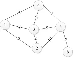
The following example illustrates the path topology diagram of the 6 sensor node, as shown in Figure 1. The source node S is the sensor 1, the destination node D is the sensor 6, the line between the nodes indicates that there is a link between them, and the number on the line represents the energy consumption of information transfer. Finding a minimum energy consumption transmission path from node 1 to node 6 is a specific goal.
Fig. 1. Path topology of 6 sensor nodes
The path-based decimal chromosome coding strategy is used to generate the initialized chromosome population randomly. Assuming that the population size is 5, the first generation of randomly generated population is shown in Figure 2. From this population, it can be seen that each chromosome satisfies the above 3 requirements.
1
4
3 5
2
6
8
9 9
2 1
3
10 9
Fig. 2. The population initialized by 6 sensor nodes
When the population is initialized, the mutation and crossover operation is performed. Then, some unlawful (unconnected) chromosomes are generated. In order to ensure that each chromosome is legitimate, a modified operation is needed. The length of each chromosome will change after the correction, but the chromosome is legal and the first and last node is the source node and the destination node, respectively. After modification operation of the above initialization population, the population shown in Figure 3 may be obtained.
Fig. 3. A possible population after evolution
4
Results
In this section, first of all, the proposed algorithm is used to make a series of experimental tests in standard DE. In order to measure its performance, the proposed algorithm is compared with the classical GA and PSO. And then the different parameter settings and DE variants are tested and compared, and the test results are analyzed. Finally, the improved crossover strategy proposed is used to improve the algorithm, and a comparative experiment is made.
4.1 Experimental environment and parameter setting
It should be noted that, except for special instructions, the unified parameter settings are as follows. Population size popsize (NP) =100, scaling factor F=1, and crossover probability Cr=0.8. The mutation method uses "DE/Rand/1", and the maximum evolution algebra (FES) is 100. If the theoretical optimal solution is found, the program terminates. All the algorithms run 100 times independently. The
1 3 2 5 4 6
1 4 5 3 2 6
1 2 4 3 5 6
1 3 4 5 2 6
1 5 2 4 3 6
Adjustment point Target node
Chromosome 1 Chromosome 2 Chromosome 3 Chromosome 4 Chromosome 5
1 3 2 5 6
1 4 5 6
1 4 3 2 5 6
1 3 4 5 6
1 2 5 6
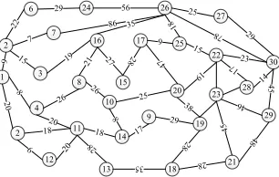
experimental environment is WinXP operating system, with hardware configured for core I3, 2.8GHzCPU, and software platform Matlab7.1. The test dataset includes 6, 20 and 30 nodes of the WSN, namely 3 different scale optimization problems. The network topology is shown in Figures 1, 4, and 5, respectively.
Fig. 4. Path topology of 20 sensor nodes
Fig. 5. Path topology of 30 sensor nodes
The theoretical minimum path values corresponding to each test dataset are shown in Table 1.
Table 1. 5 shortest path problem datasets
Problems The number of sensors The theoretical minimum values
1 6 10
2 20 142
3 30 121
4.2 Overall performance comparison
In order to verify the effectiveness of this method, the standard differential evolution algorithm is compared with the classical GA and PSO on the test set. These algorithms are all famous evolutionary algorithms and the parameter values in the source literature are used. The purpose of the experiment is to test whether the algorithm can find the theoretical minimum path for these optimal path problems, that is, the theoretical minimum path value in Table 1. The evolutionary algebra and
5 1 2 6 11 16 19 4 10 3 9 15 7 8 14 20 12 17 13 18 30
230 130 89
72
16
45 40
32 77
147
194 14 220
40 220 60 61 17 43 27 29 30 250 35 20 62 25 136 161 71 144 58 220 32 24 72 54 150 110 65 50 6 1 2 12 24 26 27 7 30 13 18 19 2 3
16 17 25
22
8 15
20 23 28
4 11 14 9 29 21 22
29 56 25
29 45 48 28 35 9 20 6 7 86 15 19 35 18 78 9 15 23 27 28 21 26 8 20 18 10 26 8 25
47 19 17
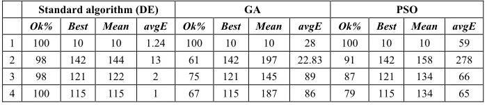
success rate that the minimum value needs are also found. The results of the experiment are shown in Table 2. In Table 2, ok% is the success rate of finding the theoretical minimum value. Best indicates the minimum value that can be found, Mean indicates the mean value of the minimum value, and avg E represents the average evolutionary algebra of the theoretical minimum. The algorithm for the best performance in the table is shown in bold type.
Table 2. Comparison between the standard DE algorithm and the classical algorithm
Standard algorithm (DE) GA PSO
Ok% Best Mean avgE Ok% Best Mean avgE Ok% Best Mean avgE
1 100 10 10 1.24 100 10 10 28 100 10 10 59
2 98 142 144 13 61 142 197 22.83 91 142 158 278
3 98 121 122 2 75 121 145 89 87 121 134 66
4 100 115 115 1 67 115 187 86 79 115 134 65
According to Table 2, from the number of full cover sets found successfully, compared with GA, the standard DE algorithm is significantly obvious than the compared algorithm on all test problems 1-4. In particular, it is found that the standard DE algorithm requires minimal evolution algebra to find the evolutionary algebra needed for theoretical value. This is due to the modified operation and mutation operation of the algorithm, which makes it possible to find the optimal solution quickly in less evolution. It can be concluded that the proposed algorithm is significantly better than the two compared algorithms. Finding the best algebraic solution has the least algebraic speed and the fastest convergence rate.
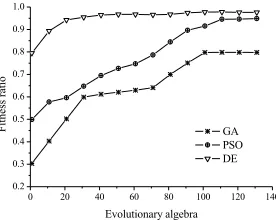
In order to further analyze the operation process of the algorithm, Figure 6 gives the evolution process of three algorithms in problem 2, in which the abscissa represents the evolutionary algebra (FES), the ordinate represents the ratio of the theoretical minimum value to the minimum value calculated. The faster the ratio is, the closer it is to 1, which shows that the algorithm can quickly get the optimal solution. Every 10 generations of the algorithm's operation results are obtained in Figure 6. Figure 6 shows that the proposed method based on the standard DE is faster than the other two methods to find the optimal solution, which benefits from the modification operation of DE algorithm and the differential evolution strategy. As a result, the original population is better than the other algorithms, and then the evolutionary algebra is the least used to find the optimal solution. The initialization population of traditional GA and PSO is randomly generated, and the initial population quality is general.
4.3 Parameter setting and mutation mode comparison
adopt a suitable mutation method and parameter configuration. Because this algorithm uses the differential operation of the set during the mutation, the value of F can only be set to 1. This section will compare Cr at different values.
Fig. 6. The evolution curve of three algorithms in test set 2
Because test problem 1 is relatively simple, all algorithms can find the theoretical minimum value in the first generation, and the probability of success can reach one hundred percent. Therefore, only the last 3 problems are tested, and each problem is run independently for 100 times. Firstly, the impact of the different crossover probability Cr on performance is tested in the "DE/rand/1" variation mode. Cr is tested every 0.1 from [0, 1], and the test results are shown in Table 3.
Table 3. Test results of DE/rand/1 mutation at different crossover probability
Standard algorithm (DE) GA PSO
Cr Ok% Best Mean avgE Ok% Best Mean avgE Ok% Best Mean avgE
0 24 142 206 1 94 121 122 1.5 88 115 120 1.8
0.1 69 142 154 21 95 121 122 1.4 98 115 116 2
0.2 79 142 152 20 94 121 123 1.3 98 115 116 1.4
0.3 95 142 146 16 95 121 122 1.5 99 115 115.3 1.7
0.4 95 142 146 15 97 121 121.3 1.4 98 115 116 1.4
0.5 98 142 144 14 96 121 121.4 1.5 99 115 115.3 1.3
0.6 97 142 145 12 100 121 121 1.2 99 115 115.3 1.3
0.7 97 142 145 12 96 121 121.4 1.4 100 115 115 1.4
0.8 98 142 144 10 98 121 121.2 1.3 100 115 115 1.2
0.9 99 142 142.4 10 96 121 121.4 1.4 99 115 115.3 1.3
1 99 142 142.3 9 95 121 121.5 1.2 100 115 115 1.7
It is pointed out in the relevant literature that the ideal F values are usually between 0.4 and 1, and a very suitable initial value is F=0.5. But this algorithm uses differential and union operations in the mutation, so the value of F can only be set to 1 by default. The crossover probability Cr controls the number of genes of individual changes in the selection process. The related research holds that, for the discrete
0 20 40 60 80 100 120 140
0.2 0.3 0.4 0.5 0.6 0.7 0.8 0.9 1.0
Fitness ratio
optimization problem, the value of Cr is more appropriate in [0, 0.3] when the optimization function is independent. On the contrary, when the function parameters are connected, Cr is more appropriate in [0.8, 1]. A very appropriate initial value is Cr=0.5. From the result of Table 3, it can be seen that the crossover probability Cr has less sensitivity to the performance of the algorithm, and it can achieve better results. Overall, when using the "DE/rand/1" mutation mode, the crossover probability Cr can achieve relatively good performance between [0.5, 0.9].
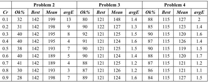
In addition, the mutation modes of "DE/best/1" and "DE/current-to-best/1" are considered, as shown in Table 4 and Table 5. When using "DE/best/1" mutation, for the test problem 2, under all different crossover probability, the success rate of finding the theoretical minimum is less than 60%, and the performance is significantly worse than that of the "DE/rand/1" mutation. For test problems 3 and 4, the performance is also slightly worse than that of the "DE/rand/1" mutation. Similarly, in the "DE/current-to-best/1" mutation, the effect of the algorithm is not as good as the "DE/rand/1" mutation, especially in problem 2 test.
Table 4. DE/rand/1 mutation mode in problem 2-4 test results
Problem 2 Problem 3 Problem 4
Cr Ok% Best Mean avgE Ok% Best Mean avgE Ok% Best Mean avgE
0.1 39 142 198 13 85 121 142 1.4 90 115 126 2
0.2 33 142 196 9 96 121 123 1.3 87 115 119 1.4
0.3 41 142 195 8 95 121 122 1.5 93 115 118 1.6
0.4 41 142 194 4 95 121 123 1.6 89 115 119 1.4
0.5 39 142 192 7 95 121 122.4 1.5 91 115 117.3 1.5
0.6 41 142 186 5 99 121 121.1 1.4 92 115 117.3 1.7
0.7 48 142 180 4 98 121 121.2 1.2 90 115 118 1.2
0.8 33 142 183 3 97 121 121.3 1.2 88 115 119 1.1
0.9 30 142 192 7 99 121 121.1 1.6 89 115 119 1.5
Table 5. DE/rand/1 mutaion in problem 2-4 test results
Problem 2 Problem 3 Problem 4
Cr Ok% Best Mean avgE Ok% Best Mean avgE Ok% Best Mean avgE
0.1 32 142 199 13 80 121 148 1.4 88 115 127 2
0.2 31 142 198 9 90 122 127 1.3 85 115 123 1.4
0.3 40 142 195 8 92 121 125 1.5 90 115 120 1.6
0.4 40 142 195 4 91 121 124 1.6 87 115 126 1.4
0.5 38 142 193 7 90 121 125 1.5 90 115 119 1.5
0.6 40 142 189 5 90 121 124 1.4 88 115 120 1.7
0.7 41 142 189 4 88 121 125 1.2 87 115 121 1.2
0.8 30 142 193 3 87 121 126 1.2 86 115 121 1.1
Therefore, according to the results of the above analysis, using the mutation strategy "DE/rand/1" mutation and Cr=0.8 as the mutation parameter, the algorithm can achieve the best performance in solving the optimal path problem.
4.4 Experimental comparison of DE-SI
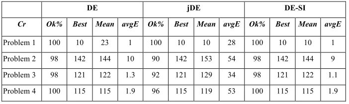
The crossover strategy is used to solve the optimization problem, and it is compared with adaptive variant jDE and standard DE. In the test, as F is fixed, the jDE algorithm only updates the parameter Cr, the parameter uses the classic jDE setting, the initial value is Cr=0.5, and the "DE/rand/1" mutation strategy is used, recorded as jDE. The contrast algorithm DE is the best standard DE, the "DE/rand/1" mutation strategy is adopted and the crossover probability is Cr=0.8. According to the SI, the strategy is combined into the classical DE as a component, and the DE-SI algorithm is obtained, recorded as DE-SI. The above three algorithms are compared with each other, and the concrete results are shown in Table 6.
Table 6. Comparison of crossover strategies and other variants
DE jDE DE-SI
Cr Ok% Best Mean avgE Ok% Best Mean avgE Ok% Best Mean avgE
Problem 1 100 10 23 1 100 10 10 28 100 10 10 1
Problem 2 98 142 144 10 90 142 153 54 98 142 144 9
Problem 3 98 121 122 1.3 92 121 129 34 98 121 122 1.1
Problem 4 100 115 115 1.9 96 115 119 53 100 115 115 1.9
From Table 6, it can be seen that the DE-SI algorithm is superior to jDE in performance and slightly better than the standard DE algorithm. Specifically, on problems 1 and 6, all algorithms can find the theoretical optimal solution. But on test problems 2 and 3, the proposed DE-SI algorithm is obviously superior to the jDE algorithm and is close to the best DE algorithm, but it is slightly better than the best DE from the convergence speed, thus verifying the effectiveness of the SI strategy.
5
Conclusion
summation operations in differential evolution. The modified operation after mutation and crossover is designed to modify the chromosomes of the existing loop and the illegal path into a legal chromosome. Finally, compared with the classical algorithm, the results verify the validity of the proposed crossover strategy (SI).
6
References
[1]Kundu, S., Das, S, Vasilakos, A.V. (2015). A modified differential evolution-based combined routing and sleep-scheduling scheme for lifetime maximization of wireless sensor networks. Soft Computing - A Fusion of Foundations, Methodologies and Applications, 19(3): 637-659.
[2]Yin, X., Ling, Z., Guan, L. (2014). Minimum distance clustering algorithm based on an improved differential evolution. International Journal of Sensor Networks, 15(1): 1-10. https://doi.org/10.1504/IJSNET.2014.059990
[3]Wang, L., Zeng, Y., Chen, T. (2015). Back propagation neural network with adaptive differential evolution algorithm for time series forecasting. Expert Systems with Applications, 42(2): 855-863. https://doi.org/10.1016/j.eswa.2014.08.018
[4]Yang, J., Zhang, H., Ling, Y. (2014). Task Allocation for Wireless Sensor Network Using Modified Binary Particle Swarm Optimization. IEEE Sensors Journal, 14(3): 882-892. https://doi.org/10.1109/JSEN.2013.2290433
[5] Li, B., Li, H., Wang, W. (2013). Performance Analysis and Optimization for Energy-Efficient Cooperative Transmission in Random Wireless Sensor Network. IEEE Transactions on Wireless Communications, 12(9): 4647-4657. https://doi.org/10.1109/ TWC.2013.072313.121949
[6]Kim, J.Y., Sharma, T., Kumar, B. (2014). Research Article Intercluster Ant Colony Optimization Algorithm for Wireless Sensor Network in Dense Environment. International Journal of Distributed Sensor Networks, 2014(5): 627-630.
[7]Iqbal, M., Naeem, M., Anpalagan, A. (2015). Wireless Sensor Network Optimization: Multi-Objective Paradigm. Sensors, 15(7): 17572-17620. https://doi.org/10.3390/ s150717572
[8]Xu, W., Zhang, Y., Shi, Q. (2015). Energy Management and Cross Layer Optimization for Wireless Sensor Network Powered by Heterogeneous Energy Sources. IEEE Transactions on Wireless Communications, 14(5): 2814-2826. https://doi.org/10.1109/TWC.2015.2394799
7
Authors
Qing Wan is a Researcher of Chongqing Vocational Institute of Engineering, Chongqing, 402260, China. His research interests include big data.
Ming-Jiang Weng and Song Liu work in Chongqing University of Posts and Telecommunication, Chongqing, China. Ming-Jiang Weng’s research interests include clustering. Song Liu research interests include network optimization.