Jarkko Isotalo
Birthweights of children during years 1965-69
5000.0 4800.0 4600.0 4400.0 4200.0 4000.0 3800.0 3600.0 3400.0 3200.0 3000.0 2800.0 2600.0 2400.0 30
20
10
0
Std. Dev = 486.32 Mean = 3553.8 N = 120.00
Horsepower
300 200
100 0
Time to Accelerate from 0 to 60 mph (sec)
30
20
10
Preface
These lecture notes have been used at Basics of Statistics course held in Uni-versity of Tampere, Finland. These notes are heavily based on the following books.
Agresti, A. & Finlay, B., Statistical Methods for the Social Sci-ences, 3th Edition. Prentice Hall, 1997.
Anderson, T. W. & Sclove, S. L., Introductory Statistical Analy-sis. Houghton Mifflin Company, 1974.
Clarke, G.M. & Cooke, D., A Basic course in Statistics. Arnold, 1998.
Electronic Statistics Textbook,
http://www.statsoftinc.com/textbook/stathome.html.
Freund, J.E.,Modern elementary statistics. Prentice-Hall, 2001. Johnson, R.A. & Bhattacharyya, G.K.,Statistics: Principles and Methods, 2nd Edition. Wiley, 1992.
Leppälä, R.,Ohjeita tilastollisen tutkimuksen toteuttamiseksi SPSS for Windows -ohjelmiston avulla, Tampereen yliopisto, Matem-atiikan, tilastotieteen ja filosofian laitos, B53, 2000.
Moore, D., The Basic Practice of Statistics. Freeman, 1997. Moore, D. & McCabe G., Introduction to the Practice of Statis-tics, 3th Edition. Freeman, 1998.
Newbold, P., Statistics for Business and Econometrics. Prentice Hall, 1995.
Weiss, N.A., Introductory Statistics. Addison Wesley, 1999.
1
The Nature of Statistics
[Agresti & Finlay (1997), Johnson & Bhattacharyya (1992), Weiss (1999), Anderson & Sclove (1974) and Freund (2001)]
1.1
What is statistics?
Statistics is a very broad subject, with applications in a vast number of different fields. In generally one can say that statistics is the methodology for collecting, analyzing, interpreting and drawing conclusions from informa-tion. Putting it in other words, statistics is the methodology which scientists and mathematicians have developed for interpreting and drawing conclu-sions from collected data. Everything that deals even remotely with the collection, processing, interpretation and presentation of data belongs to the domain of statistics, and so does the detailed planning of that precedes all these activities.
Definition 1.1 (Statistics). Statistics consists of a body of methods for
col-lecting and analyzing data. (Agresti & Finlay, 1997)
From above, it should be clear that statistics is much more than just the tabu-lation of numbers and the graphical presentation of these tabulated numbers. Statistics is the science of gaining information from numerical and categori-cal1 data. Statistical methods can be used to find answers to the questions
like:
• What kind and how much data need to be collected?
• How should we organize and summarize the data?
• How can we analyse the data and draw conclusions from it?
• How can we assess the strength of the conclusions and evaluate their uncertainty?
1Categorical data (or qualitative data) results from descriptions, e.g. the blood type
That is, statistics provides methods for
1. Design: Planning and carrying out research studies.
2. Description: Summarizing and exploring data.
3. Inference: Making predictions and generalizing about phenomena rep-resented by the data.
Furthermore, statistics is the science of dealing with uncertain phenomenon and events. Statistics in practice is applied successfully to study the effec-tiveness of medical treatments, the reaction of consumers to television ad-vertising, the attitudes of young people toward sex and marriage, and much more. It’s safe to say that nowadays statistics is used in every field of science.
Example 1.1 (Statistics in practice). Consider the following problems:
–agricultural problem: Is new grain seed or fertilizer more productive? –medical problem: What is the right amount of dosage of drug to treatment? –political science: How accurate are the gallups and opinion polls?
–economics: What will be the unemployment rate next year? –technical problem: How to improve quality of product?
1.2
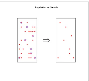
Population and Sample
Population and sample are two basic concepts of statistics. Population can be characterized as the set of individual persons or objects in which an inves-tigator is primarily interested during his or her research problem. Sometimes wanted measurements for all individuals in the population are obtained, but often only a set of individuals of that population are observed; such a set of individuals constitutes a sample. This gives us the following definitions of population and sample.
Definition 1.2 (Population). Population is the collection of all individuals
or items under consideration in a statistical study. (Weiss, 1999)
Definition 1.3 (Sample). Sample is that part of the population from which
Population vs. Sample
⇒
Figure 1: Population and Sample
Always only a certain, relatively few, features of individual person or object are under investigation at the same time. Not all the properties are wanted to be measured from individuals in the population. This observation empha-size the importance of a set of measurements and thus gives us alternative definitions of population and sample.
Definition 1.4 (Population). A (statistical) population is the set of
mea-surements (or record of some qualitive trait) corresponding to the entire col-lection of units for which inferences are to be made. (Johnson & Bhat-tacharyya, 1992)
Definition 1.5 (Sample). A sample from statistical population is the set of
measurements that are actually collected in the course of an investigation. (Johnson & Bhattacharyya, 1992)
When population and sample is defined in a way of Johnson & Bhattacharyya, then it’s useful to define the source of each measurement assampling unit, or simply, a unit.
different populations, following examples demonstrates possible discrepancies on populations.
Example 1.2 (Finite population). In many cases the population under
con-sideration is one which could be physically listed. For example: –The students of the University of Tampere,
–The books in a library.
Example 1.3 (Hypothetical population). Also in many cases the population
is much more abstract and may arise from the phenomenon under consid-eration. Consider e.g. a factory producing light bulbs. If the factory keeps using the same equipment, raw materials and methods of production also in future then the bulbs that will be produced in factory constitute a hypothet-ical population. That is, sample of light bulbs taken from current production line can be used to make inference about qualities of light bulbs produced in future.
1.3
Descriptive and Inferential Statistics
There are two major types of statistics. The branch of statistics devoted to the summarization and description of data is called descriptive statistics
and the branch of statistics concerned with using sample data to make an inference about a population of data is called inferential statistics.
Definition1.6 (Descriptive Statistics). Descriptive statistics consist of
meth-ods for organizing and summarizing information (Weiss, 1999)
Definition 1.7 (Inferential Statistics). Inferential statistics consist of
meth-ods for drawing and measuring the reliability of conclusions about population based on information obtained from a sample of the population. (Weiss, 1999)
Descriptive statistics includes the construction of graphs, charts, and tables, and the calculation of various descriptive measures such as averages, measures of variation, and percentiles. In fact, the most part of this course deals with descriptive statistics.
Example1.4 (Descriptive and Inferential Statistics). Consider event of
toss-ing dice. The dice is rolled 100 times and the results are formtoss-ing the sample data. Descriptive statistics is used to grouping the sample data to the fol-lowing table
Outcome of the roll Frequencies in the sample data
1 10
2 20
3 18
4 16
5 11
6 25
Inferential statistics can now be used to verify whether the dice is a fair or not.
Descriptive and inferential statistics are interrelated. It is almost always nec-essary to use methods of descriptive statistics to organize and summarize the information obtained from a sample before methods of inferential statistics can be used to make more thorough analysis of the subject under investi-gation. Furthermore, the preliminary descriptive analysis of a sample often reveals features that lead to the choice of the appropriate inferential method to be later used.
Sometimes it is possible to collect the data from the whole population. In that case it is possible to perform a descriptive study on the population as well as usually on the sample. Only when an inference is made about the population based on information obtained from the sample does the study become inferential.
1.4
Parameters and Statistics
Definition 1.8 (Parameters and Statistics). A parameter is an unknown
numerical summary of the population. A statistic is a known numerical sum-mary of the sample which can be used to make inference about parameters. (Agresti & Finlay, 1997)
So the inference about some specific unknown parameter is based on a statis-tic. We use known sample statistics in making inferences about unknown population parameters. The primary focus of most research studies is the pa-rameters of the population, not statistics calculated for the particular sample selected. The sample and statistics describing it are important only insofar as they provide information about the unknown parameters.
Example 1.5 (Parameters and Statistics). Consider the research problem of
finding out what percentage of 18-30 year-olds are going to movies at least once a month.
• Parameter: The proportionpof 18-30 year-olds going to movies at least once a month.
• Statistic: The proportion pˆof 18-30 year-olds going to movies at least once a month calculated from the sample of 18-30 year-olds.
1.5
Statistical data analysis
Begin
Formulate the research problem
Define population and sample
Collect the data
Do descriptive data analysis
Use appropriate statistical methods to solve the research problem
Report the results
End
2
Variables and organization of the data
[Weiss (1999), Anderson & Sclove (1974) and Freund (2001)]2.1
Variables
A characteristic that varies from one person or thing to another is called a
variable, i.e, a variable is any characteristic that varies from one individual member of the population to another. Examples of variables for humans are height, weight, number of siblings, sex, marital status, and eye color. The first three of these variables yield numerical information (yield numerical measurements) and are examples of quantitative (or numerical) vari-ables, last three yield non-numerical information (yield non-numerical mea-surements) and are examples of qualitative (or categorical) variables.
Quantitative variables can be classified as either discrete orcontinuous.
Discrete variables. Some variables, such as the numbers of children in fam-ily, the numbers of car accident on the certain road on different days, or the numbers of students taking basics of statistics course are the results of counting and thus these are discrete variables. Typically, a discrete variable is a variable whose possible values are some or all of the ordinary counting numbers like 0,1,2,3, . . .. As a definition, we can say that a variable is dis-crete if it has only a countable number of distinct possible values. That is, a variable is is discrete if it can assume only a finite numbers of values or as many values as there are integers.
Continuous variables. Quantities such as length, weight, or temperature can in principle be measured arbitrarily accurately. There is no indivible unit. Weight may be measured to the nearest gram, but it could be measured more accurately, say to the tenth of a gram. Such a variable, called continuous, is intrinsically different from a discrete variable.
2.1.1 Scales
The categories into which a qualitative variable falls may or may not have a natural ordering. For example, occupational categories have no natural ordering. If the categories of a qualitative variable are unordered, then the qualitative variable is said to be defined on a nominal scale, the word nominal referring to the fact that the categories are merely names. If the categories can be put in order, the scale is called an ordinal scale. Based on what scale a qualitative variable is defined, the variable can be called as a nominal variable or an ordinal variable. Examples of ordinal variables are education (classified e.g. as low, high) and "strength of opinion" on some proposal (classified according to whether the individual favors the proposal, is indifferent towards it, or opposites it), and position at the end of race (first, second, etc.).
Scales for Quantitative Variables. Quantitative variables, whether discrete or continuos, are defined either on an interval scale or on a ratio scale. If one can compare the differences between measurements of the variable meaningfully, but not the ratio of the measurements, then the quantitative variable is defined on interval scale. If, on the other hand, one can compare both the differences between measurements of the variable and the ratio of the measurements meaningfully, then the quantitative variable is defined on ratio scale. In order to the ratio of the measurements being meaningful, the variable must have natural meaningful absolute zero point, i.e, a ratio scale is an interval scale with a meaningful absolute zero point. For example, temperature measured on the Certigrade system is a interval variable and the height of person is a ratio variable.
2.2
Organization of the data
Observing the values of the variables for one or more people or things yield
data. Each individual piece of data is called anobservationand the collec-tion of all observacollec-tions for particular variables is called a data set ordata matrix. Data set are the values of variables recorded for a set of sampling units.
data still continues to be nominal data. Coded numerical data do not share any of the properties of the numbers we deal with ordinary arithmetic. With recards to the codes for marital status, we cannot write 3>1 or 2<4, and we cannot write 2−1 = 4−3 or1 + 3 = 4. This illustrates how important it is always check whether the mathematical treatment of statistical data is really legimatite.
Data is presented in a matrix form (data matrix). All the values of particular variable is organized to the same column; the values of variable forms the column in a data matrix. Observation, i.e. measurements collected from sampling unit, forms a row in a data matrix. Consider the situation where there are k numbers of variables andn numbers of observations (sample size is n). Then the data set should look like
Variables
Sampling units
x11 x12 x13 . . . x1k
x21 x22 x23 . . . x2k
x31 x32 x33 . . . x3k
..
. . ..
xn1 xn2 xn3 . . . xnk
where xij is a value of the j:th variable collected from i:th observation, i=
3
Describing data by tables and graphs
[Johnson & Bhattacharyya (1992), Weiss (1999) and Freund (2001)]
3.1
Qualitative variable
The number of observations that fall into particular class (or category) of the qualitative variable is called thefrequency(orcount) of that class. A table listing all classes and their frequencies is called a frequency distribution.
In addition of the frequencies, we are often interested in the percentage of a class. We find the percentage by dividing the frequency of the class by the total number of observations and multiplying the result by 100. The percentage of the class, expressed as a decimal, is usually referred to as the
relative frequency of the class.
Relative frequency of the class= Frequency in the class
Total number of observation
A table listing all classes and their relative frequencies is called a relative frequency distribution. The relative frequencies provide the most rele-vant information as to the pattern of the data. One should also state the sample size, which serves as an indicator of the creditability of the relative frequencies. Relative frequencies sum to 1 (100%).
A cumulative frequency (cumulative relative frequency) is obtained by summing the frequencies (relative frequencies) of all classes up to the specific class. In a case of qualitative variables, cumulative frequencies makes sense only for ordinal variables, not for nominal variables.
The qualitative data are presented graphically either as a pie chart or as a horizontal or vertical bar graph.
A pie chart is a disk divided into pie-shaped pieces proportional to the relative frequencies of the classes. To obtain angle for any class, we multiply the relative frequencies by 360 degrees, which corresponds to the complete circle.
whose height is equal to the frequency (or relative frequency) of the class. In a bar graph, its bars do not touch each other. At vertical bar graph, the classes are displayed on the vertical axis and the frequencies of the classes on the horizontal axis.
Nominal data is best displayed by pie chart and ordinal data by horizontal or vertical bar graph.
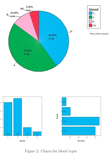
Example 3.1. Let the blood types of 40 persons are as follows:
O O A B A O A A A O B O B O O A O O A A A A AB A B A A O O A O O A A A O A O O AB
Summarizing data in a frequency table by using SPSS:
Analyze -> Descriptive Statistics -> Frequencies,
Analyze -> Custom Tables -> Tables of Frequencies
Table 1: Frequency distribution of blood types
BLOOD
16 40.0
18 45.0
4 10.0
2 5.0
40 100.0
BLOOD O A B
AB Total Valid
Frequency Percent
Statistics
Graphical presentation of data in SPSS:
Graphs -> Interactive -> Pie -> Simple,
O
A
B
AB blood
Pies show counts O
40.00% n=16
A
45.00% n=18 B 10.00%
n=4
AB 5.00%
n=2
O A B AB
blood
10% 20% 30% 40%
Percent
n=16 n=18 n=4 n=2
10% 20% 30% 40%
Percent
O A B AB
blood
n=16 n=18 n=4 n=2
3.2
Quantitative variable
The data of the quantitative variable can also presented by a frequency dis-tribution. If the discrete variable can obtain only few different values, then the data of the discrete variable can be summarized in a same way as quali-tative variables in a frequency table. In a place of the qualiquali-tative categories, we now list in a frequency table the distinct numerical measurements that appear in the discrete data set and then count their frequencies.
If the discrete variable can have a lot of different values or the quantitative variable is the continuous variable, then the data must be grouped into classes (categories) before the table of frequencies can be formed. The main steps in a process of grouping quantitative variable into classes are:
(a) Find the minimum and the maximum values variable have in the data set
(b) Choose intervals of equal length that cover the range between the min-imum and the maxmin-imum without overlapping. These are called class intervals, and their end points are calledclass limits.
(c) Count the number of observations in the data that belongs to each class interval. The count in each class is the class frequency.
(c) Calculate the relative frequencies of each class by dividing the class frequency by the total number of observations in the data.
The number in the middle of the class is called class markof the class. The number in the middle of the upper class limit of one class and the lower class limit of the other class is called the real class limit. As a rule of thumb, it is generally satisfactory to group observed values of numerical variable in a data into 5 to 15 class intervals. A smaller number of intervals is used if number of observations is relatively small; if the number of observations is large, the number on intervals may be greater than 15.
If quantitative data is discrete with only few possible values, then the variable should graphically be presented by a bar graph. Also if some reason it is more reasonable to obtain frequency table for quantitative variable with unequal class intervals, then variable should graphically also be presented by a bar graph!
Example 3.2. Age (in years) of 102 people:
34,67,40,72,37,33,42,62,49,32,52,40,31,19,68,55,57,54,37,32, 54,38,20,50,56,48,35,52,29,56,68,65,45,44,54,39,29,56,43,42, 22,30,26,20,48,29,34,27,40,28,45,21,42,38,29,26,62,35,28,24, 44,46,39,29,27,40,22,38,42,39,26,48,39,25,34,56,31,60,32,24, 51,69,28,27,38,56,36,25,46,50,36,58,39,57,55,42,49,38,49,36, 48,44
Summarizing data in a frequency table by using SPSS:
Analyze -> Descriptive Statistics -> Frequencies,
Analyze -> Custom Tables -> Tables of Frequencies
Table 2: Frequency distribution of people’s age
Frequency distribution of people's age
6 5.9 5.9
10 9.8 15.7
14 13.7 29.4
11 10.8 40.2
19 18.6 58.8
8 7.8 66.7
12 11.8 78.4
12 11.8 90.2
4 3.9 94.1
2 2.0 96.1
4 3.9 100.0
102 100.0
18 - 22 23 - 27 28 - 32 33 - 37 38 - 42 43 - 47 48 - 52 53 - 57 58 - 62 63 - 67 68 - 72 Total Valid
Frequency Percent
Cumulative Percent
Graphical presentation of data in SPSS:
Graphs -> Interactive -> Histogram,
Age (in years)
67.5 - 72.5 62.5 - 67.5 57.5 - 62.5 52.5 - 57.5 47.5 - 52.5 42.5 - 47.5 37.5 - 42.5 32.5 - 37.5 27.5 - 32.5 22.5 - 27.5 17.5 - 22.5
Frequencies
20
10
0
Figure 3: Histogram for people’s age
Example 3.3. Prices of hotdogs ($/oz.):
0.11,0.17,0.11,0.15,0.10,0.11,0.21,0.20,0.14,0.14,0.23,0.25,0.07, 0.09,0.10,0.10,0.19,0.11,0.19,0.17,0.12,0.12,0.12,0.10,0.11,0.13, 0.10,0.09,0.11,0.15,0.13,0.10,0.18,0.09,0.07,0.08,0.06,0.08,0.05, 0.07,0.08,0.08,0.07,0.09,0.06,0.07,0.08,0.07,0.07,0.07,0.08,0.06, 0.07,0.06
Table 3: Frequency distribution of prices of hotdogs
Frequencies of prices of hotdogs ($/oz.)
5 9.3 9.3
19 35.2 44.4
15 27.8 72.2
6 11.1 83.3
3 5.6 88.9
4 7.4 96.3
1 1.9 98.1
1 1.9 100.0
54 100.0 0.031-0.06 0.061-0.09 0.091-0.12 0.121-0.15 0.151-0.18 0.181-0.21 0.211-0.24 0.241-0.27 Total Valid Frequency Percent Cumulative Percent or alternatively
Table 4: Frequency distribution of prices of hotdogs (Left Endpoints Ex-cluded, but Right Endpoints Included)
Frequencies of prices of hotdogs ($/oz.)
5 9.3 9.3
19 35.2 44.4
15 27.8 72.2
6 11.1 83.3
3 5.6 88.9
4 7.4 96.3
1 1.9 98.1
1 1.9 100.0
54 100.0 0.03-0.06 0.06-0.09 0.09-0.12 0.12-0.15 0.15-0.18 0.18-0.21 0.21-0.24 0.24-0.27 Total Valid Frequency Percent Cumulative Percent
Price ($/oz)
.270 - .300 .240 - .270 .210 - .240 .180 - .210 .150 - .180 .120 - .150 .090 - .120 .060 - .090 .030 - .060 0.000 - .030 20
10
0
Figure 4: Histogram for prices
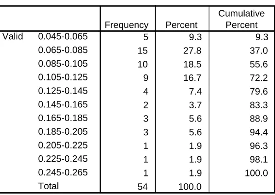
Table 5: Frequency distribution of prices of hotdogs
Frequencies of prices of hotdogs ($/oz.)
5 9.3 9.3
15 27.8 37.0
10 18.5 55.6
9 16.7 72.2
4 7.4 79.6
2 3.7 83.3
3 5.6 88.9
3 5.6 94.4
1 1.9 96.3
1 1.9 98.1
1 1.9 100.0
54 100.0 0.045-0.065 0.065-0.085 0.085-0.105 0.105-0.125 0.125-0.145 0.145-0.165 0.165-0.185 0.185-0.205 0.205-0.225 0.225-0.245 0.245-0.265 Total Valid Frequency Percent Cumulative Percent Price ($/oz)
.265 - .285 .245 - .265 .225 - .245 .205 - .225 .185 - .205 .165 - .185 .145 - .165 .125 - .145 .105 - .125 .085 - .105 .065 - .085 .045 - .065 .025 - .045
Frequencies 16 14 12 10 8 6 4 2 0
Another types of graphical displays for quantitative data are
(a) dotplot
Graphs -> Interactive -> Dot
(b) stem-and-leaf diagram of juststemplot
Analyze -> Descriptive Statistics -> Explore
(c) frequency and relative-frequency polygon for frequencies and for relative frequencies (Graphs -> Interactive -> Line)
(d) ogives for cumulative frequencies and for cumulative relative frequen-cies (Graphs -> Interactive -> Line)
3.3
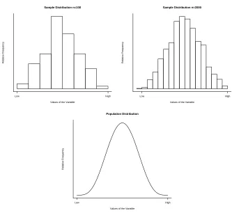
Sample and Population Distributions
Frequency distributions for a variable apply both to a population and to sam-ples from that population. The first type is called thepopulation distribu-tion of the variable, and the second type is called a sample distribution. In a sense, the sample distribution is a blurry photograph of the population distribution. As the sample size increases, the sample relative frequency in any class interval gets closer to the true population relative frequency. Thus, the photograph gets clearer, and the sample distribution looks more like the population distribution.
Sample Distribution n=100
Values of the Variable
Relative Frequency
Low High
Sample Distribution n=2000
Values of the Variable
Relative Frequency
Low High
Population Distribution
Values of the Variable
Relative Frequency
Low High
Figure 6: Sample and Population Distributions
One way to summarize a sample of population distribution is to describe its shape. A group for which the distribution is bell-shaped is fundamentally different from a group for which the distribution is U-shaped, for example.
U−shaped
Values of the Variable
Relative Frequency
Low High
Bell−shaped
Values of the Variable
Relative Frequency
Low High
Figure 7: U-shaped and Bell-shaped Frequency Distributions
Skewed to the right
Values of the Variable
Relative Frequency
Low High
Skewed to the left
Values of the Variable
Relative Frequency
Low High
4
Measures of center
[Agresti & Finlay (1997), Johnson & Bhattacharyya (1992), Weiss (1999) and Anderson & Sclove (1974)]
Descriptive measures that indicate where the center or the most typical value of the variable lies in collected set of measurements are called measures of center. Measures of center are often referred to as averages.
The median and the mean apply only to quantitative data, whereas the mode can be used with either quantitative or qualitative data.
4.1
The Mode
The sample modeof a qualitative or a discrete quantitative variable is that value of the variable which occurs with the greatest frequency in a data set. A more exact definition of the mode is given below.
Definition 4.1 (Mode). Obtain the frequency of each observed value of the
variable in a data and note the greatest frequency.
1. If the greatest frequency is 1 (i.e. no value occurs more than once), then the variable has no mode.
2. If the greatest frequency is 2 or greater, then any value that occurs with that greatest frequency is called a sample mode of the variable.
To obtain the mode(s) of a variable, we first construct a frequency distribu-tion for the data using classes based on single value. The mode(s) can then be determined easily from the frequency distribution.
Example 4.1. Let us consider the frequency table for blood types of 40
persons.
We can see from frequency table that the mode of blood types is A.
The mode in SPSS:
Table 6: Frequency distribution of blood types BLOOD 16 40.0 18 45.0 4 10.0 2 5.0 40 100.0 BLOOD O A B AB Total Valid Frequency Percent Statistics
When we measure a continuous variable (or discrete variable having a lot of different values) such as height or weight of person, all the measurements may be different. In such a case there is no mode because every observed value has frequency 1. However, the data can be grouped into class intervals and the mode can then be defined in terms of class frequencies. With grouped quantitative variable, the mode class is the class interval with highest fre-quency.
Example 4.2. Let us consider the frequency table for prices of hotdogs
($/oz.): Then the mode class is 0.065-0.085.
Table 7: Frequency distribution of prices of hotdogs
Frequencies of prices of hotdogs ($/oz.)
5 9.3 9.3
15 27.8 37.0
10 18.5 55.6
9 16.7 72.2
4 7.4 79.6
2 3.7 83.3
3 5.6 88.9
3 5.6 94.4
1 1.9 96.3
1 1.9 98.1
1 1.9 100.0
4.2
The Median
The sample median of a quantitative variable is that value of the variable in a data set that divides the set of observed values in half, so that the observed values in one half are less than or equal to the median value and the observed values in the other half are greater or equal to the median value. To obtain the median of the variable, we arrange observed values in a data set in increasing order and then determine the middle value in the ordered list.
Definition 4.2 (Median). Arrange the observed values of variable in a data
in increasing order.
1. If the number of observation is odd, then the sample median is the observed value exactly in the middle of the ordered list.
2. If the number of observation is even, then the sample median is the number halfway between the two middle observed values in the ordered list.
In both cases, if we let n denote the number of observations in a data set, then the sample median is at position n+12 in the ordered list.
Example 4.3. 7 participants in bike race had the following finishing times
in minutes: 28,22,26,29,21,23,24. What is the median?
Example 4.4. 8 participants in bike race had the following finishing times
in minutes: 28,22,26,29,21,23,24,50. What is the median?
The median in SPSS:
Analyze -> Descriptive Statistics -> Frequencies
4.3
The Mean
The most commonly used measure of center for quantitative variable is the (arithmetic) sample mean. When people speak of taking an average, it is mean that they are most often referring to.
Definition 4.3 (Mean). The sample mean of the variable is the sum of
observed values in a data divided by the number of observations.
Example 4.5. 7 participants in bike race had the following finishing times
in minutes: 28,22,26,29,21,23,24. What is the mean?
Example 4.6. 8 participants in bike race had the following finishing times
in minutes: 28,22,26,29,21,23,24,50. What is the mean?
The mean in SPSS:
Analyze -> Descriptive Statistics -> Frequencies,
Analyze -> Descriptive Statistics -> Descriptives
To effectively present the ideas and associated calculations, it is convenient to represent variables and observed values of variables by symbols to prevent the discussion from becoming anchored to a specific set of numbers. So let us use xto denote the variable in question, and then the symbol xi denotes
ith observation of that variable in the data set.
If the sample size is n, then the mean of the variable x is
x1+x2 +x3+· · ·+xn
n .
To further simplify the writing of a sum, the Greek letter P
(sigma) is used as a shorthand. The sum x1 +x2+x3+· · ·+xn is denoted as
n
X
i=1
xi,
and read as "the sum of allxi with iranging from 1 ton". Thus we can now
Definition 4.4. The sample mean of the variable is the sum of observed
values x1, x2, x3, . . . , xn in a data divided by the number of observations n.
The sample mean is denoted by x¯, and expressed operationally,
¯
x=
Pn
i=1xi
n or
P
xi
n .
4.4
Which measure to choose?
The mode should be used when calculating measure of center for the qualita-tive variable. When the variable is quantitaqualita-tive with symmetric distribution, then the mean is proper measure of center. In a case of quantitative variable with skewed distribution, the median is good choice for the measure of cen-ter. This is related to the fact that the mean can be highly influenced by an observation that falls far from the rest of the data, called an outlier.
5
Measures of variation
[Johnson & Bhattacharyya (1992), Weiss (1999) and Anderson & Sclove (1974)]
In addition to locating the center of the observed values of the variable in the data, another important aspect of a descriptive study of the variable is numerically measuring the extent of variation around the center. Two data sets of the same variable may exhibit similar positions of center but may be remarkably different with respect to variability.
Just as there are several different measures of center, there are also several different measures of variation. In this section, we will examine three of the most frequently used measures of variation; thesample range, the sample interquartile range and the sample standard deviation. Measures of variation are used mostly only for quantitative variables.
5.1
Range
The sample range is obtained by computing the difference between the largest observed value of the variable in a data set and the smallest one.
Definition 5.1 (Range). The sample range of the variable is the difference
between its maximum and minimum values in a data set: Range=Max−Min.
The sample range of the variable is quite easy to compute. However, in using the range, a great deal of information is ignored, that is, only the largest and smallest values of the variable are considered; the other observed values are disregarded. It should also be remarked that the range cannot ever decrease, but can increase, when additional observations are included in the data set and that in sense the range is overly sensitive to the sample size.
Example 5.1. 7 participants in bike race had the following finishing times
in minutes: 28,22,26,29,21,23,24. What is the range?
Example 5.2. 8 participants in bike race had the following finishing times
Example 5.3. Prices of hotdogs ($/oz.):
0.11,0.17,0.11,0.15,0.10,0.11,0.21,0.20,0.14,0.14,0.23,0.25,0.07, 0.09,0.10,0.10,0.19,0.11,0.19,0.17,0.12,0.12,0.12,0.10,0.11,0.13, 0.10,0.09,0.11,0.15,0.13,0.10,0.18,0.09,0.07,0.08,0.06,0.08,0.05, 0.07,0.08,0.08,0.07,0.09,0.06,0.07,0.08,0.07,0.07,0.07,0.08,0.06, 0.07,0.06
The range in SPSS:
Analyze -> Descriptive Statistics -> Frequencies,
Analyze -> Descriptive Statistics -> Descriptives
Table 8: The range of the prices of hotdogs
Range of the prices of hotdogs
54 .20 .05 .25
54 Price ($/oz)
Valid N (listwise)
N Range Minimum Maximum
5.2
Interquartile range
Before we can define the sample interquartile range, we have to first define the percentiles, the deciles and the quartiles of the variable in a data set. As was shown in section 4.2, the median of the variable divides the observed values into two equal parts – the bottom 50% and the top 50%. The percentiles of the variable divide observed values into hundredths, or 100 equal parts. Roughly speaking, the first percentile, P1, is the number
that divides the bottom 1% of the observed values from the top 99%; second percentile, P2, is the number that divides the bottom 2% of the observed
values from the top 98%; and so forth. The median is the 50th percentile.
The deciles of the variable divide the observed values into tenths, or 10 equal parts. The variable has nine deciles, denoted by D1, D2, . . . , D9. The first
decile D1 is 10th percentile, the second decile D2 is the 20th percentile, and
so forth.
variable has three quartiles, denoted by Q1, Q2 and Q3. Roughly speaking,
the first quartile, Q1, is the number that divides the bottom 25% of the
observed values from the top 75%; second quartile, Q2, is the median, which
is the number that divides the bottom 50% of the observed values from the top 50%; and the third quartile, Q3, is the number that divides the bottom
75% of the observed values from the top 25%.
At this point our intuitive definitions of percentiles and deciles will suffice. However, quartiles need to be defined more precisely, which is done below.
Definition 5.2 (Quartiles). Let n denote the number of observations in a
data set. Arrange the observed values of variable in a data in increasing order.
1. The first quartile Q1 is at position n+14 ,
2. The second quartile Q2 (the median) is at position n+12 ,
3. The third quartile Q3 is at position 3(n4+1),
in the ordered list.
If a position is not a whole number, linear interpolation is used.
Next we define the sample interquartile range. Since the interquartile range is defined using quartiles, it is preferred measure of variation when the median is used as the measure of center (i.e. in case of skewed distribution).
Definition 5.3 (Interquartile range). The sample interquartile rangeof the
variable, denoted IQR, is the difference between the first and third quartiles of the variable, that is,
IQR=Q3 −Q1.
Roughly speaking, the IQR gives the range of the middle 50% of the observed values.
Example 5.4. 7 participants in bike race had the following finishing times
in minutes: 28,22,26,29,21,23,24. What is the interquartile range?
Example 5.5. 8 participants in bike race had the following finishing times
in minutes: 28,22,26,29,21,23,24,50. What is the interquartile range?
Example 5.6. The interquartile range for prices of hotdogs ($/oz.) in SPSS:
Analyze -> Descriptive Statistics -> Explore
Table 9: The interquartile range of the prices of hotdogs
Interquartile Range of the prices of hotdogs
.0625 Interquartile Range
Price ($/oz)
Statistic
5.2.1 Five-number summary and boxplots
Minimum, maximum and quartiles together provide information on center and variation of the variable in a nice compact way. Written in increas-ing order, they comprise what is called the five-number summary of the variable.
Definition 5.4 (Five-number summary). The five-number summary of the
variable consists of minimum, maximum, and quartiles written in increasing order:
Min, Q1, Q2, Q3,Max.
Aboxplotis based on the five-number summary and can be used to provide a graphical display of the center and variation of the observed values of variable in a data set. Actually, two types of boxplots are in common use – boxplot and modified boxplot. The main difference between the two types of boxplots is that potentialoutliers(i.e. observed value, which do not appear to follow the characteristic distribution of the rest of the data) are plotted individually in a modified boxplot, but not in a boxplot. Below is given the procedure how to construct boxplot.
1. Determine the five-number summary
2. Draw a horizontal (or vertical) axis on which the numbers obtained in step 1 can be located. Above this axis, mark the quartiles and the minimum and maximum with vertical (horizontal) lines.
3. Connect the quartiles to each other to make a box, and then connect the box to the minimum and maximum with lines.
The modified boxplot can be constructed in a similar way; except the poten-tial outliers are first identified and plotted individually and the minimum and maximum values in boxplot are replace with theadjacent values, which are the most extreme observations that are not potential outliers.
Example 5.7. 7 participants in bike race had the following finishing times
in minutes: 28,22,26,29,21,23,24. Construct the boxplot.
Example 5.8. The five-number summary and boxplot for prices of hotdogs
($/oz.) in SPSS:
Analyze -> Descriptive Statistics -> Descriptives
Table 10: The five-number summary of the prices of hotdogs
Five-number summary
Price ($/oz)
54 0 .1000 .05 .25 .0700 .1000 .1325 Valid
Missing N
Median Minimum Maximum
25 50 75 Percentiles
Graphs -> Interactive -> Boxplot,
0.05 0.10 0.15 0.20 0.25
Price ($/oz)
Figure 9: Boxplot for the prices of hotdogs
5.3
Standard deviation
The sample standard deviation is the most frequently used measure of vari-ability, although it is not as easily understood as ranges. It can be considered as a kind of average of the absolute deviations of observed values from the mean of the variable in question.
Definition 5.6 (Standard deviation). For a variablex, the sample standard
deviation, denoted by sx (or when no confusion arise, simply by s), is
sx =
s
Pn
i=1(xi−x)¯ 2
n−1 .
Since the standard deviation is defined using the sample mean x¯ of the vari-able x, it is preferred measure of variation when the mean is used as the measure of center (i.e. in case of symmetric distribution). Note that the stardard deviation is always positive number, i.e., sx ≥0.
from the mean,
n
X
i=1
(xi−x)¯ 2 = (x1 −x)¯ 2 + (x2−x)¯ 2+· · ·+ (xn−x)¯ 2,
is called sum of squared deviations and provides a measure of total de-viation from the mean for all the observed values of the variable. Once the sum of squared deviations is divided by n−1, we get
s2x =
Pn
i=1(xi−x)¯ 2
n−1 ,
which is called the sample variance. The sample standard deviation has following alternative formulas:
sx =
s
Pn
i=1(xi−x)¯ 2
n−1 (1)
=
s
Pn
i=1x2i −n¯x2
n−1 (2)
=
s
Pn
i=1x2i −(
Pn
i=1xi)2/n
n−1 . (3)
The formulas (2) and (3) are useful from the computational point of view. In hand calculation, use of these alternative formulas often reduces the arith-metic work, especially when x¯turns out to be a number with many decimal places.
The more variation there is in the observed values, the larger is the standard deviation for the variable in question. Thus the standard deviation satisfies the basic criterion for a measure of variation and like said, it is the most commonly used measure of variation. However, the standard deviation does have its drawbacks. For instance, its values can be strongly affected by a few extreme observations.
Example 5.9. 7 participants in bike race had the following finishing times
in minutes: 28,22,26,29,21,23,24.
What is the sample standard deviation?
Example 5.10. The standard deviation for prices of hotdogs ($/oz.) in
SPSS:
Analyze -> Descriptive Statistics -> Frequencies,
Table 11: The standard deviation of the prices of hotdogs
Standard deviation of the prices of hotdogs
54 .1113 .04731 .002
54 Price ($/oz)
Valid N (listwise)
N Mean Std. Deviation Variance
5.3.1 Empirical rule for symmetric distributions
For bell-shaped symmetric distributions (like the normal distribu-tion), empirical rule relates the standard deviation to the proportion of the observed values of the variable in a data set that lie in a interval around the mean x¯.
Empirical guideline for symmetric bell-shaped distribution, approximately
68% of the values lie within x¯±sx,
95% of the values lie within x¯±2sx,
99.7% of the values lie within x¯±3sx.
5.4
Sample statistics and population parameters
Of the measures of center and variation, the sample mean x¯and the sample standard deviation s are the most commonly reported. Since their values depend on the sample selected, they vary in value from sample to sample. In this sense, they are calledrandom variables to emphasize that their values vary according to the sample selected. Their values are unknown before the sample is chosen. Once the sample is selected and they are computed, they become known sample statistics.
We shall regularly distinguish between sample statistics and the correspond-ing measures for the population. Section 1.4 introduced the parameter for a summary measure of the population. A statistic describes a sample, while a parameter describes the population from which the sample was taken.
Definition 5.7 (Notation for parameters). Let µ and σ denote the mean
We call µ and σ the population mean and population standard devi-ation The population mean is the average of the population measurements. The population standard deviation describes the variation of the population measurements about the population mean.
6
Probability Distributions
[Agresti & Finlay (1997), Johnson & Bhattacharyya (1992), Moore & McCabe (1998) and Weiss (1999)]
Inferential statistical methods use sample data to make predictions about the values of useful summary descriptions, called parameters, of the popu-lation of interest. This chapter treats parameters as known numbers. This is artificial, since parameter values are normally unknown or we would not need inferential methods. However, many inferential methods involve com-paring observed sample statistics to the values expected if the parameter values equaled particular numbers. If the data are inconsistent with the par-ticular parameter values, the we infer that the actual parameter values are somewhat different.
6.1
Probability distributions
We first define the term probability, using a relative frequency approach. Imagine a hypothetical experiment consisting of a very long sequence of re-peated observations on somerandom phenomenon. Each observation may or may not result in some particular outcome. The probability of that outcome is defined to be the relative frequency of its occurence, in the long run.
Definition 6.1 (Probability). The probability of a particular outcome is
the proportion of times that outcome would occur in a long run of repeated observations.
A simplified representation of such an experiment is a very long sequence of flips of a coin, the outcome of interest being that a head faces upwards. Any on flip may or may not result in a head. If the coin is balanced, then a basic result in probability, called law of large numbers, implies that the proportion of flips resulting in a head tends toward 1/2 as the number of flips increases. Thus, the probability of a head in any single flip of the coin equals 1/2
Definition 6.2 (Random variable). A random variable is a variable whose
value is a numerical outcome of a random phenomenon.
We usually denote random variables by capital letters near the end of the alphabet, such as X or Y. Some values of the random variable X may be more likely than others. The probability distribution of the random variable X lists the the possible outcomes together with their probabilities the variable X can have.
The probability distribution of adiscrete random variableX assigns a prob-ability to each possible values of the variable. Each probprob-ability is a number between 0 and 1, and the sum of the probabilities of all possible values equals 1. Let xi, i= 1,2, . . . , k, denote a possible outcome for the random variable
X, and let P(X =xi) =P(xi) =pi denote the probability of that outcome.
Then
0≤P(xi)≤1 and
k
X
i=1
P(xi) = 1
since each probability falls between 0 and 1, and since the total probability equals 1.
Definition 6.3 (Probability distribution of a discrete random variable). A
discrete random variable X has a countable number of possible values. The probability distribution of X lists the values and their probabilities:
Value of X x1 x2 x3 . . . xk
Probability P(x1) P(x2) P(x3) . . . P(xk)
The probabilities P(xi) must satisfy two requirements:
1. Every probability P(xi) is a number between0 and 1.
2. P(x1) +P(x2) +· · ·+P(xk) = 1.
We can use aprobability histogramto picture the probability distribution of a discrete random variable. Furthermore, we can find the probability of any event [such as P(X ≤ xi) or P(xi ≤ X ≤ xj), i ≤ j] by adding the
Example 6.1. The instructor of a large class gives 15% each of 5=excellent,
20% each of 4=very good, 30% each of 3=good, 20% each of 2=satisfactory, 10% each of 1=sufficient, and 5% each of 0=fail. Choose a student at random from this class. The student’s grade is a random variable X. The value of
X changes when we repeatedly choose students at random, but it is always one of 0,1,2,3,4 or 5.
What is the probability distribution of X?
Draw a probability histogram for X.
What is the probability that the student got 4=very good or better, i.e,
P(X ≥4)?
Continuous random variable X, on the other hand, takes all values in some interval of numbers between a and b. That is, continuous random variable has a continuum of possible values it can have. Let x1 and x2, x1 ≤ x2,
denote possible outcomes for the random variable X which can have values in the interval of numbers between a and b. Then clearly both x1 andx2 are
belonging to the interval of a and b, i.e.,
x1 ∈[a, b] and x2 ∈[a, b],
and x1 and x2 themselves are forming the interval of numbers [x1, x2]. The
probability distribution of a continuous random variable X then assigns a probability to each of these possible interval of numbers [x1, x2]. The
prob-ability that random variable X falls in any particular interval [x1, x2] is a
number between 0 and 1, and the probability of the interval[a, b], containing all possible values, equals 1. That is, it is required that
0≤P(x1 ≤X ≤x2)≤1 and P(a≤X ≤b) = 1.
Definition 6.4 (Probability distribution of a continuous random variable).
A continuous random variable X takes all values in an interval of numbers
[a, b]. The probability distribution of X describes the probabilities P(x1 ≤
X ≤x2) of all possible intervals of numbers [x1, x2].
The probabilities P(x1 ≤X ≤x2) must satisfy two requirements:
1. For every interval[x1, x2], the probabilityP(x1 ≤X ≤x2) is a number
2. P(a≤X ≤b) = 1.
The probability model for a continuous random variable assign probabilities to intervals of outcomes rather than to individual outcomes. In fact, all continuous probability distributions assign probability 0 to every individual outcome.
The probability distribution of a continuous random variable is pictured by a density curve. A density curve is smooth continuous curve having area exactly 1 underneath it such like curves representing the population distri-bution in section 3.3. In fact, the population distribution of a variable is, equivalently, the probability distribution for the value of that variable for a subject selected randomly from the population.
Example 6.2.
Probabilities of continuous random variable
Event x1<X<x2
Density
x1 x2
P(x1<X<x2)
6.2
Mean and standard deviation of random variable
Like a population distribution, a probability distribution of a random variable has parameters describing its central tendency and variability. The mean describes central tendency and thestandard deviation describes variability of the random variableX. The parameter values are the values these measures would assume, in the long run, if we repeatedly observed the values the random variable X is having.
The mean and the standard deviation of the discrete random variable are defined in the following ways.
Definition 6.5 (Mean of a discrete random variable). Suppose that X is a
discrete random variable whose probability distribution is Value of X x1 x2 x3 . . . xk
Probability P(x1) P(x2) P(x3) . . . P(xk)
The mean of the discrete random variable X is
µ=x1P(x1) +x2P(x2) +x3P(x3) +· · ·+xkP(xk)
=
k
X
i=1
xiP(xi).
The meanµ is also called theexpected valueof X and is denoted by E(X).
Definition 6.6 (Standard deviation of a discrete random variable). Suppose
that X is a discrete random variable whose probability distribution is Value of X x1 x2 x3 . . . xk
Probability P(x1) P(x2) P(x3) . . . P(xk)
and that µ is the mean ofX. The variance of the discrete random variable
X is
σ2 = (x1 −µ)2P(x1) + (x2−µ)2P(x2) + (x3−µ)2P(x3) +· · ·+ (xk−µ)2P(xk)
=
k
X
i=1
(xi −µ)2P(xi).
Example 6.3. In an experiment on the behavior of young children, each
subject is placed in an area with five toys. The response of interest is the number of toys that the child plays with. Past experiments with many sub-jects have shown that the probability distribution of the number X of toys played with is as follows:
Number of toys xi 0 1 2 3 4 5
Probability P(xi) 0.03 0.16 0.30 0.23 0.17 0.11
Calculate the mean µ and the standard deviation σ.
The mean and standard deviation of a continuous random variable can be calculated, but to do so requires more advanced mathematics, and hence we do not consider them in this course.
6.3
Normal distribution
A continuous random variable graphically described by a certain bell-shaped density curve is said to have the normal distribution. This distribution is the most important one in statistics. It is important partly because it approximates well the distributions of many variables. Histograms of sample data often tend to be approximately bell-shaped. In such cases, we say that the variable is approximately normally distributed. The main reason for its prominence, however, is that most inferential statistical methods make use of properties of the normal distribution even when the sample data are not bell-shaped.
A continuous random variable X following normal distribution has two pa-rameters: the mean µand the standard deviation σ.
Definition 6.7 (Normal distribution). A continuous random variable X is
said to be normally distributed or to have a normal distribution if its density curve is a symmetric, bell-shaped curve, characterized by its mean µ and standard deviation σ. For each fixed number z, the probability concentrated within interval [µ − zσ, µ +zσ] is the same for all normal distributions. Particularly, the probabilities
P(µ−σ < X < µ+σ) = 0.683 (4)
P(µ−2σ < X < µ+ 2σ) = 0.954 (5)
hold. A random variable X following normal distribution with a mean of µ
and a standard deviation of σ is denoted by X ∼N(µ, σ).
There are other symmetric bell-shaped density curves that are not normal. The normal density curves are specified by a particular equation. The height of the density curve at any point x is given by the density function
f(x) = 1
σ√2πe
−12(x−µ
σ )
2
. (7)
We will not make direct use of this fact, although it is the basis of math-ematical work with normal distribution. Note that the density function is completely determined by µand σ.
Example 6.4.
Normal Distribution
Values of X
Density
µ −3σ µ −2σ µ − σ µ µ + σ µ +2σ µ +3σ
Figure 11: Normal distribution.
Definition 6.8 (Standard normal distribution). A continuous random
Thestandard normal tablecan be used to calculate probabilities concern-ing the random variable Z. The standard normal table gives area to the left of a specified value of z under density curve:
P(Z ≤z) =Area under curve to the left ofz.
For the probability of an interval [a, b]:
P(a≤Z ≤b) = [Area to left ofb]−[Area to left ofa].
The following properties can be observed from the symmetry of the standard normal distribution about 0:
(a) P(Z ≤0) = 0.5,
(b) P(Z ≤ −z) = 1−P(Z ≤z) =P(Z ≥z).
Example 6.5.
(a) Calculate P(−0.155< Z <1.60).
(b) Locate the value z that satisfies P(Z > z) = 0.25.
If the random variable X is distributed as X ∼N(µ, σ), then the standard-ized variable
Z = X−µ
σ (8)
has the standard normal distribution. That is, if X is distributed as X ∼
N(µ, σ), then
P(a≤X ≤b) =P
a−µ
σ ≤Z ≤
b−µ
σ
, (9)
where Z has the standard normal distribution. This property of the normal distribution allows us to cast probability problem concerning X into one concerning Z.
Example 6.6. The number of calories in a salad on the lunch menu is
nor-mally distributed with mean µ = 200 and standard deviation σ = 5. Find the probability that the salad you select will contain:
(a) More than 208 calories.
7
Sampling distributions
[Agresti & Finlay (1997), Johnson & Bhattacharyya (1992), Moore & McCabe (1998) and Weiss (1999)]
7.1
Sampling distributions
Statistical inference draws conclusions about population on the basis of data. The data are summarized by statistics such as the sample mean and the sample standard deviation. When the data are produced by random sam-pling or randomized experimentation, a statistic is a random variable that obeys the laws of probability theory. The link between probability and data is formed by the sampling distributions of statistics. A sampling distribution shows how a statistic would vary in repeated data production.
Definition 7.1 (Sampling distribution). A sampling distribution is a
prob-ability distribution that determines probabilities of the possible values of a sample statistic. (Agresti & Finlay 1997)
Each statistic has a sampling distribution. A sampling distribution is simply a type of probability distribution. Unlike the distributions studied so far, a sampling distribution refers not to individual observations but to the values of statistic computed from those observations, in sample after sample.
Sampling distribution reflect the sampling variability that occurs in collecting data and using sample statistics to estimate parameters. A sampling distri-bution of statistic based on n observations is the probability distribution for that statistic resulting from repeatedly taking samples of size n, each time calculating the statistic value. The form of sampling distribution is often known theoretically. We can then make probabilistic statements about the value of statistic for one sample of some fixed size n.
7.2
Sampling distributions of sample means
Select an simple random sample of sizen from population, and measure a variable X on each individual in the sample. The data consist of observa-tions on n random variables X1, X2, . . . , Xn. A single Xi is a measurement
on one individual selected at random from the population and therefore Xi
is a random variable with probability distribution equalling the population distribution of variableX. If the population is large relatively to the sample, we can consider X1, X2, . . . , Xn to be independent random variables each
having the same probability distribution. This is our probability model for measurements on each individual in an simple random sample.
The sample mean of an simple random sample of size n is
¯
X = X1+X2+· · ·+Xn
n .
Note that we now use notation X¯ for the sample mean to emphasize that X¯
is random variable. Once the values of random variables X1, X2, . . . , Xn are
observed, i.e., we have values x1, x2, . . . , xn in our use, then we can actually
compute the sample mean x¯ in usual way.
If the population variable X has a population mean µ, the µis also mean of each observation Xi. Therefore, by the addition rule for means of random
variables,
µX¯ =E( ¯X) =E
X1+X2+· · ·+Xn
n
= E(X1+X2+· · ·+Xn)
n
= E(X1) +E(X2) +· · ·+E(Xn)
n
= µX1 +µX2 +· · ·+µXn
n
= µ+µ+· · ·+µ
n
=µ.
That is, the mean ofX¯ is the same as the population meanµof the variable
random variables, X¯ has the variance
σX2¯ =
σ2
X1 +σ
2
X2 +· · ·+σ
2
Xn
n2
= σ
2+σ2+· · ·+σ2
n2
= σ
2
n,
and hence the standard deviation of X¯ is
σX¯ = √σ
n.
The standard deviation of X¯ is also called the standard error of X¯.
Key Fact7.1 (Mean and standard error ofX¯). For a random sample of size
n from a population having mean µ and standard deviation σ, the sampling distribution of the sample mean X¯ has meanµX¯ =µand standard deviation,
i.e., standard error σX¯ = √σ
n. (Moore & McCabe, 1998)
The mean and standard error of X¯ shows that the sample mean X¯ tends to be closer to the population mean µfor larger values ofn, since the sampling distribution becomes less spead about µ. This agrees with our intuition that larger samples provide more preciseestimates of population characteristics.
Example 7.1. Consider the following population distribution of the variable
X:
Values of X 2 3 4
Relative frequencies of X 13 13 13
and let X1 and X2 to be random variables following the probability
distribu-tion of populadistribu-tion distribudistribu-tion of X.
(a) Verify that the population mean and population variance are
µ= 3, σ2 = 2
3.
(b) Construct the probability distribution of the sample mean X¯.
(Johnson & Bhattacharyya 1992)
We have above described the center and spread of the probability distribution of a sample mean X¯, but not its shape. The shape of the distribution X¯
depends on the shape of the population distribution. Special case is when population distribution is normal.
Key Fact 7.2 (Distribution of sample mean). Suppose a variable X of a
population is normally distributed with mean µ and standard deviation σ. Then, for samples of size n, the sample meanX¯ is also normally distributed and has mean µ and standard deviation √σ
n. That is, if X ∼ N(µ, σ), then
¯
X ∼N(µ, σ
√
n). (Weiss, 1999)
Example7.2.Consider a normal population with meanµ= 82and standard
deviation σ= 12.
(a) If a random sample of size 64 is selected, what is the probability that the sample mean X¯ will lie between 80.8and 83.2?
(b) With a random sample of size 100, what is the probability that the sample mean X¯ will lie between 80.8 and 83.2?
(Johnson & Bhattacharyya 1992)
When sampling from nonnormal population, the distribution of X¯ depends on what is the population distribution of the variableX. A surprising result, known as the central limit theorem states that when the sample size n
is large, the probability distribution of the sample mean X¯ is approximately normal, regardless of the shape of the population distribution.
Key Fact 7.3 (Central limit theorem). Whatever is the population
distri-bution of the variable X, the probability distribution of the sample mean X¯
is approximately normal when n is large. That is, when n is large, then
¯
X approximately N
µ,√σ
n
.
(Johnson & Bhattacharyya 1992)
Example 7.3.
U−shaped
Values of the Variable
Relative Frequency
Low High
Distribution of sample mean (n=100)
Values of mean
Frequency
0.40 0.45 0.50 0.55 0.60
0
5
10
15
8
Estimation
[Agresti & Finlay (1997), Johnson & Bhattacharyya (1992), Moore & McCabe (1998) and Weiss (1999)]
In this section we consider how to use sample data to estimate unknown population parameters. Statistical inference uses sample data to form two types of estimators of parameters. A point estimate consists of a sin-gle number, calculated from the data, that is the best sinsin-gle guess for the unknown parameter. A interval estimate consists of a range of numbers around the point estimate, within which the parameter is believed to fall.
8.1
Point estimation
The object of point estimation is to calculate, from the sample data, a single number that is likely to be close to the unknown value of the population parameter. The available information is assumed to be in the form of a random sample X1, X2, . . . , Xn of size n taken from the population. The
object is to formulate a statistic such that its value computed from the sample data would reflect the value of the population parameter as closely as possible.
Definition 8.1. A point estimator of a unknown population parameter is
a statistic that estimates the value of that parameter. A point estimate of a parameter is the value of a statistic that is used to estimate the parameter. (Agresti & Finlay, 1997 and Weiss, 1999)
For instance, to estimate a population mean µ, perhaps the most intuitive point estimator is the sample mean:
¯
X = X1+X2+· · ·+Xn
n .
Once the observed values x1, x2, . . . , xn of the random variablesXi are
avail-able, we can actually calculate the observed value of the sample mean x¯, which is called a point estimate of µ.
For example, the mean of the sampling distribution of the sample mean X¯
equals µ. Thus, X¯ is an unbiased estimator of the population mean µ.
A second preferable property for an estimator is a small standard error. An estimator whose standard error is smaller than those of other potential estimators is said to beefficient. An efficient estimator is desirable because, on the average, it falls closer than other estimators to the parameter. For example, it can be shown that under normal distribution, the sample mean is an efficient estimator, and hence has smaller standard error compared, e.g, to the sample median.
8.1.1 Point estimators of the population mean and standard de-viation
The sample mean X¯ is the obvious point estimator of a population mean
µ. In fact, X¯ is unbiased, and it is relatively efficient for most population distributions. It is the point estimator, denoted by µˆ, used in this text:
ˆ
µ= ¯X = X1+X2+· · ·+Xn
n .
Moreover, the sample standard deviationsis the most popular point estimate of the population standard deviation σ. That is,
ˆ
σ =s=
s
Pn
i=1(xi −x)¯ 2
n−1 .
8.2
Confidence interval
For point estimation, a single number lies in the forefront even though a standard error is attached. Instead, it is often more desirable to produce an interval of values that is likely to contain the true value of the unknown parameter.
Definition 8.2 (Confidence interval). A confidence interval for a parameter
is a range of numbers within which the parameter is believed to fall. The probability that the confidence interval contains the parameter is called the confidence coefficient. This is a chosen number close to 1, such as 0.95 or 0.99. (Agresti & Finlay, 1997)
8.2.1 Confidence interval for µ when σ known
We first confine our attention to the construction of a confidence interval for a population mean µ assuming that the population variable X is normally distributed and its the standard deviationσ isknown.
Recall the Key Fact 7.1 that when the population is normally distributed, the distribution of X¯ is also normal, i.e., X¯ ∼N(µ,√σ
n). The normal table
shows that the probability is 0.95 that a normal random variable will lie within 1.96 standard deviations from its mean. For X¯, we then have
P(µ−1.96√σ
n <X < µ¯ + 1.96
σ
√
n) = 0.95.
Now the relation
µ−1.96√σ
n <X¯ equals µ <X¯ + 1.96 σ
√n
and
¯
X < µ+ 1.96√σ
n equals X¯ −1.96 σ
√
n < µ.
Hence the probability statement
P(µ−1.96√σ
n <X < µ¯ + 1.96
σ
√
n) = 0.95
can also be expressed as
P( ¯X−1.96√σ
n < µ <X¯ + 1.96
σ
√
n) = 0.95.
This second form tells us that the ran