Lecture 10-Assiciation Rules-M

(1)

CSC479

Data Mining

Lecture # 9

Mining Frequent Patterns

(2)

(3)

Mining Frequent Itemsets

TID Items

1 Bread, Milk

(4)

The itemset

lattice

null

AB AC AD AE BC BD BE CD CE DE

A B C D E

ABC ABD ABE ACD ACE ADE BCD BCE BDE CDE

ABCD ABCE ABDE ACDE BCDE

ABCDE

Given d items, there are

2d _{possible itemsets}

(5)

The Apriori Principle

Apriori

principle (Main observation):

–

If an itemset is

frequent

, then all of its

subsets

must

also be frequent

–

If an itemset is

not frequent

, then all of its

supersets

cannot be frequent

–

The support of an itemset

never exceeds

the

support of its subsets

–

This is known as the

anti-monotone

property of

support

)

(

)

(

)

(

:

,

Y

X

Y

s

X

s

Y

X







(6)

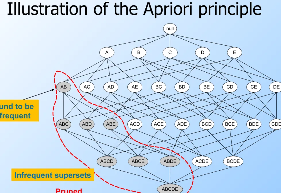
Illustration of the Apriori principle

(7)

Illustration of the Apriori principle

Found to be Infrequent

null

A B C D E

ABC ABD ABE ACD ACE ADE BCD BCE BDE CDE

ABCDE null

A B C D E

ABC ABD ABE ACD ACE ADE BCD BCE BDE CDE

ABCDE Pruned

(8)

R. Agrawal, R. Srikant: "Fast Algorithms for Mining Association Rules",

Proc. of the 20th Int'l Conference on Very Large Databases, 1994.

The Apriori algorithm

Level-wise approach

C

k

=

candidate

itemsets of size

k

L

_k

=

frequent

itemsets of size

k

Candidate generation

Frequent itemset generation

1.

k = 1

,

C

₁

= all items

2. While

C

_k

not empty

3. Scan the database to find which itemsets

in

C

_k

are

frequent

and put them into

L

_k

4. Use

L

_k

to generate a collection of

candidate

itemsets

C

_k+1

of size

k+1

(9)

Candidate Generation



Basic principle (Apriori):



An itemset of size

k+1

is candidate to be

frequent only if

all

of its subsets of size

k

are known to be frequent



Main idea:



Construct a

candidate

of size

k+1

by

combining

two

frequent

itemsets of size

k



Prune

the generated

k+1

-itemsets that do

(10)

Mining Association Rules

Example:

Beer } Diaper , Milk {  4 . 0 5 2 | T | ) Beer Diaper, , Milk ( __ 



s 67 . 0 3 2 ) Diaper , Milk ( ) Beer Diaper, Milk, ( __ 



c



Association Rule

– An implication expression of the form

X  Y, where X and Y are itemsets

– {Milk, Diaper}  {Beer}



Rule Evaluation Metrics

– Support (s)

 _{Fraction of transactions that contain}_both_X

and Y = the probability P(X,Y) that X and Y

occur together

– Confidence (c)

 How often Y appears in transactions that

contain X = the conditional probability P(Y| X) that Y occurs given that X has

occurred.

TID Items

1 Bread, Milk

2 Bread, Diaper, Beer, Eggs 3 Milk, Diaper, Beer, Coke 4 Bread, Milk, Diaper, Beer 5 Bread, Milk, Diaper, Coke



Problem Definition

– Input A set of transactions T, over a set of items I, minsup, minconf values

(11)

Mining Association Rules



Two-step approach:

1.

Frequent Itemset Generation

–

Generate all itemsets whose

support



minsup

2.

Rule Generation

–

Generate

high confidence

rules from each

frequent itemset, where each rule is a

partitioning of a frequent itemset into

Left-Hand-Side (

LHS

) and Right-Hand-Side (

RHS

)

(12)

Association Rule anti-monotonicity



Confidence is

anti-monotone

w.r.t. number

of items on the

RHS

of the rule (or

monotone

with respect to the

LHS

of the

rule)



e.g.,

L = {A,B,C,D}:

(13)

Rule Generation for APriori Algorithm

 Candidate rule is generated by merging two rules that share the same

prefix

in the RHS

 join(CDAB,BDAC)

would produce the candidate rule D  ABC

 Prune rule D  ABC if its

subset ADBC does not have high confidence

 Essentially we are doing APriori on the RHS

BD->

A

C

CD->

A

B

(14)

Closed Itemset



An itemset is closed if

none

of its immediate

supersets

has the

same

support

as the itemset

(15)

Maximal vs Closed Itemsets

Frequent Itemsets

Closed Frequent

Itemsets

Maximal Frequent

(16)

Pattern Evaluation



Association rule algorithms tend to produce too many

rules but many of them are

uninteresting

or

redundant

Redundant if {A,B,C}  {D} and {A,B}  {D} have same support

& confidence

•Summarization techniques

Uninteresting, if the pattern that is revealed does not offer useful

information.

•Interestingness measures: a hard problem to define



Interestingness measures

can be used to prune/rank the

derived patterns

Subjective measures: require human analyst Objective measures: rely on the data.



In the original formulation of association rules, support &

(17)

Computing Interestingness Measure



Given a rule

X



Y

, information needed to compute rule

interestingness can be obtained from a

contingency table

f₁₁ f₁₀ f₁₊ f₀₁ f₀₀ f_o+ f₊₁ f₊₀ N

Contingency table

for

X



Y

f

₁₁

: support of

X

and

Y

f

₁₀

: support of

X

and

Y

f

₀₁

: support of

X

and

Y

f

₀₀

: support of

X

and

Y

Used to define various measures



support, confidence, lift, Gini,

J-measure, etc.

: itemset X appears in tuple : itemset Y appears in tuple

(18)

Drawback of Confidence

Coffee Coffee

Tea

15

5

20

Tea

75

5

80

90

10

100

Association Rule:

Tea



Coffee

Confidence= P(Coffee|Tea) =

0.75

but P(Coffee) =

0.9

•

Although confidence is high, rule is misleading

•

P(Coffee|Tea) = 0.9375

Number of people that drink coffee and tea

Number of people that drink coffee but not tea

Number of people that drink coffee

(19)

Statistical Independence



Population of 1000 students



600 students know how to

swim (S)



bike

(B)



swim

and

bike

(

S

,

B

)



P(S



B)

= 420/1000 = 0.42



P(S)



P(B)

= 0.6



0.7 = 0.42

(20)

Statistical Independence





swim (S)



bike (B)



500

students know how to

swim

and

bike

(

S

,

B

)



P(S



B)

= 500/1000 =

0.5



P(S)



P(B)

= 0.6



0.7 = 0.42

(21)

Statistical Independence





swim (S)



bike (B)



300

students know how to

swim

and bike (

S

,

B

)



P(S



B)

= 300/1000 =

0.3



P(S)



P(B)

= 0.6



0.7 = 0.42

(22)

(23)

Example: Lift/Interest

Coffee Coffee

Tea

15

5

20

Tea

75

5

80

90

10

100

Association Rule: Tea



Coffee

Confidence= P(Coffee|Tea) =

0.75

but P(Coffee) =

0.9



Lift

= 0.75/0.9=

0.8333

(< 1, therefore is negatively associated)

(24)

Another Example

of the of, the

Fraction of

documents 0.9 0.9 0.8

P

(

of , the

)

≈ P

(

of

)

P

(

the

)

If I was creating a document by picking words randomly, (of, the) have more or less the same probability of appearing together by chance

hong kong hong, kong

Fraction of

documents 0.2 0.2 0.19

P

(

hong ,kong

)

≫

P

(

hong

)

P

(

kong

)

(hong, kong) have much lower probability to appear together by chance. The two words appear almost always only together

obama karagounis obama, karagounis Fraction of

documents 0.2 0.2 0.001

(obama, karagounis) have much higher probability to appear together

by chance. The two words appear almost never together

No correlation

Positive correlation

(25)

Drawbacks of Lift/Interest/Mutual

Information

honk konk honk, konk Fraction of

documents 0.0001 0.0001 0.0001

𝑀𝐼

(

h

𝑜𝑛𝑘

,

𝑘𝑜𝑛𝑘

)

=

0.0001

∗

0.0001

=

10000

hong kong hong,

kong Fraction of

documents 0.2 0.2 0.19

𝑀𝐼

(

h

𝑜𝑛𝑔

,

𝑘𝑜𝑛𝑔

)

=

0.19

0.2

∗

0.2

=

4.75