INTELIGENCIA ARTIFICIAL
http://journal.iberamia.org/
Building Dynamic Lexicons
for Sentiment Analysis
Nicol´
as Mechulam, Dami´
an Salvia, Aiala Ros´
a, Mathias Etcheverry
Instituto de Computaci´on, Facultad de Ingenier´ıa, Universidad de la Rep´ublica. Uruguay [email protected]Abstract: Nowadays, many approaches for Sentiment Analysis (SA) rely on affective lexicons to identify emotions transmitted in opinions. However, most of these lexicons do not consider that a word can express different sentiments in different predication domains, introducing errors in the sentiment inference. Due to this problem, we present a model based on a context-graph which can be used for building domain specific sentiment lexicons (DL: Dynamic Lexicons) by propagating the valence of a few seed words. For different corpora, we compare the results of a simple rule-based sentiment classifier using the corresponding DL, with the results obtained using a general affective lexicon. For most corpora containing specific domain opinions, the DL reaches better results than the general lexicon.
Keywords: Lexicon Induction, Sentiment Analysis, Natural Language Processing.
1
Introduction
Sentiment Analysis identifies and extracts opinions in order to classify their sentiments. According to Taboada et al. (2011), sentiment can be induced by lexicon based approaches, or supervised text classification, eventually including lexicon based features. Generally, the sentiment is inferred by applying heuristics or machine learning methods on texts, eventually using sentiment information of words, such as sentiment lexicon.
The basic structure of sentiment lexicons is a reduced and selected set of words with their valence (sentiment or affection, e.g. ‘bad’ as negative or ‘good’ as positive). Many classification algorithms take this dictionary as input for identifying the sentiment of a whole text or for improving the results obtained by machine-learning techniques. Even though its use is necessary, usually it is not enough.
As Levin (1991) says, the lexicon usage “has often proved to be a bottleneck in the design of large-scale natural language systems”. This fact, despite technological advances from the last two decades, is still being a problem for creating and applying this kind of resources because of heterogeneous and ambiguous word’s meaning. For instance, Ros´a et al. (2017) remarks that the use of sentiment lexicons does not produce significant improvements in sentiment prediction.
According to Pang and Lee (2008), when we face a lexicon construction problem, we must define as a first step which will be the lexicon’s units. There are many options to achieve this goal depending on text-preprocessing cost and sentiment dissipation from same-meaning lexical variations (i.e. by token, by
ISSN: 1137-3601 (print), 1988-3064 (on-line) c
word, by lemma, by stem). For example, ‘Educated’ and ‘educaaated’ tokens refers to ‘educated’ word, this word and ‘educating’ word refers to ‘educate’ lemma, and this lemma with ‘educative’ lemma refers to ‘educ’ stem. Note how sentiment is grouped when lexical unit is more general, but it requires more preprocessing on each lexical treatment.
Once lexical units are defined, we should define how sentiment is expressed and how lexical items will be retrieved. For the first problem, according to Jurafsky and Martin (2017), sentiments can be expressed in three ways: in a discrete domain (or categorical), in a continuous domain (a real number), or by vectors (where each component represents a sentiment feature). The same authors, for the second problem, say that there are two main approaches for retrieving relevant words and their sentiment: 1) by manual inference (human annotator/s), and 2) by machine learning strategies. The first family presents high accuracy with a considerable human effort, while the second one leads to a wider lexical coverage.
The process of building sentiment lexicons is a complex task because there is not a ‘universal receipt’ that indicates how sentiment is expressed. In consequence, these kinds of resources have been built by linguistics or experts, and it is hard to achieve high coverage in any context. For example, the word ‘long’ expresses opposite sentiments in the sentences “it is a long road to get there” and “a long weekend is coming”. In the first case, ‘long’ expresses a negative opinion over ‘the travel time’, and in the second example it expresses a positive opinion over ‘the weekend duration’. Also, on the same predication domain, there can be conflicting phrases (e.g. ‘low’ in “low price” and “low salary” for financial domain), or there can be phrases influenced by valence shifters (e.g. negation in ‘it’s not clean’ really means ‘it’s dirty’).
In this paper we present a method for the automatic construction of affective lexicons. For this, we estimate the valence of words accor ding to their contexts and to the domain on which opinions are expressed. We call these lexicons Dynamic Lexicons. Despite the method was tested only for Spanish, its nature makes it language-independent.
The remaining document is structured in four main sections. Section 2 corresponds to related works that present some novelty about lexicon inference, Section 3 describes the bases of the generation model, Section 4 shows empirical results and Section 5 concludes the work made.
2
Related work
Liu (2012) exposes four problems when using lexicons for predicting sentiments: 1) Opposite affection depending on the opinion object (e.g. ‘big’ is positive for capacity but negative for electronic devices), 2) Opinions without affection words (e.g. “last night my phone got wet” is negative but it does not have any key word), 3) Neutral sentences with affection word (e.g. questions like “will my phone have a good signal there?”), and 4) Sarcasm/irony sentences (e.g. “what a good phone I bought! Two days it works...”). The problem becomes more complex when combining other linguistic phenomena, such as: intonation in written text (e.g. emojis or words as ‘EXCELLENT’ or ‘eeeexcelent’) (Muhammad et al., 2013), intensification/negation (e.g. ‘tiniest’) (Polanyi and Zaenen, 2006), or when treating global vs. local sentiment (e.g. “it’s a good phone with a bad design”) (Pang and Lee, 2008).
Hatzivassiloglou and McKeown (1997) propose one of the first methods for inducing a sentiment lexicon of adjectives. Their system starts from 1336 seed words with known valence assuming there are some conjunctions that preserve the valence (e.g. ‘and’) and others that invert it (e.g. ‘but’). They report a precision of 82.05%.
Wu and Wen (2010) try to infer the polarity of ambiguous adjectives. They propose the concept of sentiment expectation that relates a noun (with known valence) with an adjective. For instance, if ‘salary’ has positive expectation, then ‘low’ should be negative-like in the phrase “the salary is low” due this phrase is negative. The authors report 80.06% of macro-F measure and 79.72% of accuracy.
Turney and Littman (2002) use PMI (Pointwise Mutual Information) and LSA (Latent Semantic Analysis) as a semi-supervised mechanism, reporting 74% of precision. Probably, the most important fact of their work is that they use only two seeds, one of each class (‘excelent’ and ‘poor’). Also, the nature of the applied method (PMI+LSA) encapsulates domain-specific information from the corpora used to build the lexicon.
Kamps et al. (2004) useWordNetto find word synonyms from a set of seeds in order to propagate their valence, or invert them when they are antonyms. The valence assigned to new words is calculated by a function called EVA (short for ‘evaluation’) which measures the distance between ‘good’ and ‘bad’ adjectives. The authors report 68.19% of precision.
Esuli and Sebastiani (2007) also useWordNet to build SentiWordNet, but they build a graph based on word’s glosses and then apply a modified version of PageRank algorithm over it. For evaluation they use Kendall Correlation measure, reporting 0.324 for positive words and 0.284 for negative words.
Another work inspired inWordNetis Hamilton et al. (2016), who introduceSentProp. They build a graph using word embeddings where each word is a node connected with their k-nearest neighbors in the semantic word space model. Then, they apply a label-propagation mechanism over the valence from a few seed words following a probabilistic model defined on the weight of each edge. They report 86.7% of accuracy, 68.8 % of f-measure and 0.4 of Kendall correlation.
Chen and Skiena (2014) build a graph with semantic inter-language edges using a variety of linguistic resources, starting from an English sentiment lexicon as seeds. They cover 136 different languages and evaluate their results using existing non-English sentiment lexicons.
Our method is inspired by these graph based approaches. We take the idea of building a word’s graph in order to propagate the valence of a few seed words (with known valence) through it. However, our method differs from them in the fact that edges in our graph represent syntagmatic co-occurrence of words in texts from a specific domain, instead of representing semantic relations between words, provided by resources such asWordNetor word embeddings.
3
Our Approach
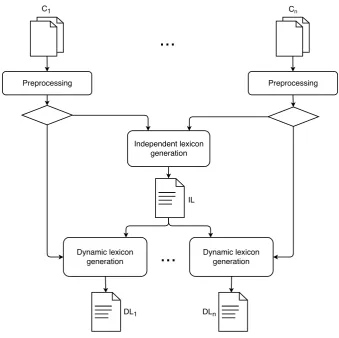
Our work is based on the following hypothesis: “the sentiment of a word depends on its context”. Such context should be understood by 1) the neighbor words (or textual context), 2) the negation influ-ence, and 3) the predication domain. In these terms, we create a mechanism for building a lexicon of
<word,valence>pairs based on the architecture described in Figure 1.
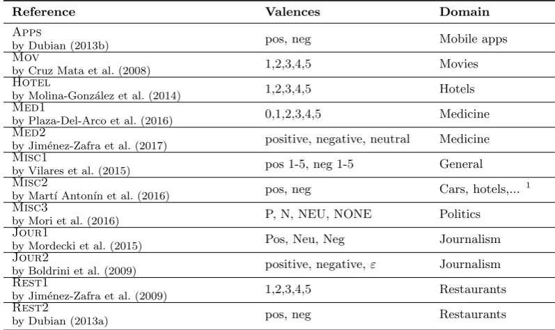
We started from a set of diverse corpus (C1,...,Cn) with sentiment-tagged opinions (e.g. reviews from
movies, sports, restaurants, etc.), described in Tables 1 and 2 – refer to the author’s paper for further information (annotation method, valence meaning, etc). The complete corpus has 79.643 opinions. Each corpus was preprocessed applying word correction and lemmatization, identifying negated words and standardizing their heterogeneous valences.
To detect words within a negation scope we trained a bidirectional long-short term memory network using the SFU-NEG corpus (Mart´ı Anton´ın et al., 2016). The inputs of the neural model are word embeddings built using skip-gram on a Spanish corpus of almost six billion words Azzinnari and Mart´ınez (2016). More details on these experiments can be found in Salvia and Mechulam (2018).
After these preprocessing steps, we used the 10% of each corpus to build an Independent Lexicon (IL) where words sentiment does not depend on the context to which the words belong, they are always positive or negative.
From the remaining corpora, we used 72% of each corpusCi to build eachDynamic Lexicon (DLi),
using the words of the IL as seeds. The dynamic lexicon is built by generating a context-graph and applying a semi-supervised valence propagation mechanism over it.
We used the remaining 18% of eachCi as test corpus. To evaluate we compared the results obtained
using the domain specific generated lexicon against a general purpose lexicon in sentiment analysis de-tection.
In the following, we describe the mechanisms applied to build theILand theDL.
3.1
Independent Lexicon
We built anIndependent Lexicon(IL) taking the ideas of Ghag and Shah (2014). These authors propose Senti-TFIDF, a mechanism which treats sentiments as a Bag-of-Words (BoW). The result will be a lexicon where word’s sentiment is independent of the context, since it includes words that are frequently used
C1
Independent lexicon generation
Cn
Preprocessing
Dynamic lexicon generation
Dynamic lexicon generation
...
Preprocessing
...
DL1
IL
DLn
Figure 1: Architecture
with the same polarity in the different domains we studied. These words are used as seeds for sentiment propagation, in the construction of the dynamic lexicon. In this work, despite we know when a word is negated or not, we modify the original mechanism to include the negation in the calculus, resulting in the following equations:
X-TFt,d=
(
ft+,d ifd∈DX
ft−,d ifd∈DX
P
x∈DXft+,x+
P
x∈DXft−,x
X-IDFt= log
|DX∪DX|
|{d∈DX:t+∈d} ∪ {d∈DX:t−∈d}|
whereXrepresents theP OSorN EGclass andX the complementary class ofX; besides,t−/t+represent
if termt is negated or not, respectively. The words in theIL will be the top 150 with higher absolute value of TF-IDF (product of both formulas).
Taking a portion of the resources described in Table 1 (as it was detailed in the introduction of this chapter), we built anILlimited to 150 words, including 75 positive words and 75 negative words. For instance, the most representative words on each category were desastre (‘disaster’), as negative, and excelente(‘excellent’), as positive.
3.2
Dynamic Lexicon
Reference Valences Domain
Apps
by Dubian (2013b) pos, neg Mobile apps
Mov
by Cruz Mata et al. (2008) 1,2,3,4,5 Movies
Hotel
by Molina-Gonz´alez et al. (2014) 1,2,3,4,5 Hotels
Med1
by Plaza-Del-Arco et al. (2016) 0,1,2,3,4,5 Medicine
Med2
by Jim´enez-Zafra et al. (2017) positive, negative, neutral Medicine
Misc1
by Vilares et al. (2015) pos 1-5, neg 1-5 General
Misc2
by Mart´ı Anton´ın et al. (2016) pos, neg Cars, hotels,... 1
Misc3
by Mori et al. (2016) P, N, NEU, NONE Politics
Jour1
by Mordecki et al. (2015) Pos, Neu, Neg Journalism
Jour2
by Boldrini et al. (2009) positive, negative,ε Journalism
Rest1
by Jim´enez-Zafra et al. (2009) 1,2,3,4,5 Restaurants
Rest2
by Dubian (2013a) pos, neg Restaurants
Table 1: Collected corpus with sentiment annotation by domain
Corpus Total IL(10%) DL(72%) Eval(18%)
Apps 8.281 828 7.453 1.491
Mov 3.878 388 3.490 698
Hotel 1.816 182 1.634 327
Med1 743 74 669 134
Med2 453 45 408 82
Misc1 3.600 360 3.240 648
Misc2 400 40 360 72
Misc3 2.466 247 2.219 444
Jour1 2.260 226 2.034 407
Jour2 974 97 877 175
Rest1 2.202 220 1.982 396
Rest2 52.570 5.257 47.313 9.463
Total 79.643 7.964 71.679 14.337
Table 2: Corpus sizes after splitting for IL, DL and Evaluation.
3.2.1 Context Graph
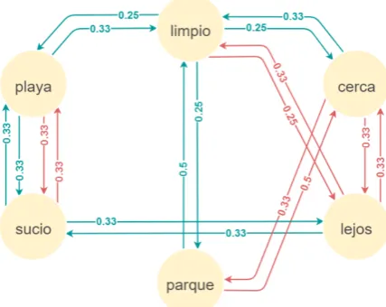
The idea behind the construction of theContext Graph, inspired by the semantic graphs used in (Kamps et al., 2004; Esuli and Sebastiani, 2007; Hamilton et al., 2016; Santos et al., 2012), is that nodes represent the vocabulary of the domain, and edges represent the textual contexts (contiguous words in the text). For instance, if the words ‘A’ and ‘B’ appear together in the text, then there is an edge<A, B>in the graph, representing anadjacency relation. Each specific corpus will be associated to a graph from which a DLwill be obtained. Thus, a context graph will be derived from each particular domain.
Normally, in sentences like “The sky is turning red”, the words ‘The’ and ‘is’ lack lexical content, and their occurrence avoids adjacency relations such as ‘sky’ - ‘beautiful’. To solve this issue we decided to discard stop words and auxiliary verbs.
Figure 2: Context graph of a simple corpus.
its lemma and, in this way, decrease the sparsity without losing affective content.
The presence of negations in the text affects the valence of the words within its scope. Since the context graph seeks to model the contexts of words, negations are an additional aspect to be represented in the structure.
To model the negation, we decided to maintain two types of relationships: ((direct)) and ((inverse)). However, the affection transmitted by the relationships<no-X,Y >and< X, no-Y >is the same. That is, considering “The dog that does not bite is good” and “The dog that bites is not good”, the relations between ((bites)) and ((good)) is assumed to express the same sentiment, although the sentences are semantically different2.
Formally, direct relations (< x,y >dir) are understood as links between two neighboring words with
the same affective value (both are denied or none are). On the other hand, an inverse relation (< x,
y >inv) is one in which the neighboring words have a different affective value (one has the opposite value
than the other one). In these conditions, for the first case, the valence is maintained, while the second is inverted.
Although for a set of texts the graph reflects the words contexts, it does not take into account the frequency with which they occur. That is, assuming that the words<dog, bites>co-occur more frequently than<dog, plays>, the former should take more importance in the representation, since ‘dog’ is closely related to ‘bites’ and probably has a similar affective value. For this reason, we decided to apply a weighting mechanism based on the number of co-occurrences in the texts, the weight (w) of an edge is the probability that two words are adjacent (directly or indirectly).
It is important to note that the probabilityP(y|x) depends on the relation of the node “x”. Therefore, since the weight of< x, y >and< y, x >could take different values, there is a need to express the origin and destination of the relation. Consequently, the context graph must be directed in order to adequately represent the weights. Given that there exist direct and inverse relations, the context graph is a directed graph with multiple weighted edges.
In figure 2 we show the context graph resulting from the following corpus, designed to explain the concept:
• La playa es sucia y est´a lejos. / The beach is dirty and far.
• El parque es limpio y no est´a lejos. / The park is clean and it is not far.
• La playa est´a limpia y es cerca. / The beach is clean and near.
• El parque no est´a cerca, est´a lejos. / The park is not near, it is far.
• La playa no est´a sucia. / The beach is not dirty.
As we can see,sucia/sucio(dirty) andlimpia/limpio(clean) are represented by a unique node, labeled with the corresponding lemma (sucio andlimpio). Stop words (el, la) and auxiliary verbs (es, est´a) are not included in the graph. Green edges indicate direct relations while red ones indicate inverse relations. Each edge weight is computed dividing the number of co-occurrences of its endpoints (distinguishing negated and non-negated contexts) by the number of occurrences of its origin. In order to illustrate this, we analyze the three occurrences of the lemmaplaya:
• the first one is in the non-negated context ofsucio, generating a direct edge (green) with a weight of 0.33 (1/3) between the nodesplaya andsucio,
• the second one is in the negated context ofsucio, hence an inverse edge (red) with a weight of 0.33 (1/3) is added,
• the last one is in the non-negated context oflimpio, resulting in a direct edge (green) with a weight of 0.33 (1/3).
3.2.2 Valence Propagation
In this section, we describe the algorithm used for valence propagation over the context graph. This algorithm allows us to obtain the valence of each node of thecontext graph, starting from the seeds (IL), whose affective value is known. The result of this algorithm will determine theDL.
The algorithm is based on the concept of influence (inf), a positive real value that represents how similar is the valence of a node respect to another. This value is given by the path that maximizes the product of the edges. It is calculated recursively according to Equation 1, whereinreturns the incident nodes to the target. Notice how the function, when looking for the incidents of the destination node (in(y)), implicitly calculates the maximum path from x to y. To clarify this idea, the Example 3.1 is proposed (for simplicity the bidirectionality of the edges is omitted).
inf(x, y) =
(
1 : ifx=y
max
z∈in(y)
inf(x, z)∗ω(< z, y >) : else (1)
Example 3.1. Given the following simplified context graph, it is shown the calculation (top-down) of the influence of node S (seed) towards node C.
inf(S, C) = max
inf(S, A)∗ω(< A, C >)
inf(S, B)∗ω(< B, C >)
= max
inf(S, S)∗ω(< S, A >)∗ω(< A, C >)
inf(S, S)∗ω(< S, B >)∗ω(< B, C >)
= max
1∗0.7∗0.5 = 0.35 1∗0.3∗0.5 = 0.15
Note that Example 3.1 does not include inverse edges. This simplification is intentional since the Equation1 only describes the influence of direct relations. Remember that a direct relation represents two neighboring words with the same sentiment, while an inverse relation represents words with opposite sentiments. In this sense, it is necessary to define direct influence (infdir) and inverse influence
(infinv) in a mutually recursive way according to the Equation 2
infdir(x, y) =
1 : ifx=y
max
z∈in(y)
infdir(x, z)∗ω(< z, y >dir)
infinv(x, z)∗ω(< z, y >inv)
: else
infinv(x, y) =
0 : ifx=y
max
z∈in(y)
infdir(x, z)∗ω(< z, y >inv)
infinv(x, z)∗ω(< z, y >dir)
: else
(2)
It is important to note that thedirect influence of a node on itself is 1 since a word always has the same valence as itself. Analogously, the inverse influence of a node on itself is 0 since a word never has a valence opposite to itself. As a way to analyze the influence calculations with this new formula, Example 3.2 is proposed. A real context graph is much more complex, for this reason an algorithm inspired by Dijkstra was designed to optimize the calculations.
Example 3.2. Given the following context graph, the calculation (bottom-up) of the direct and inverse influences from the node S (seed) to node C is shown.
Node S (base step)
infdir(S, S) = 1
infinv(S, S) = 0 Node A
infdir(S, A) = max
infdir(S, S)∗ω(< S, A >dir)
infinv(S, S)∗ω(< S, A >inv)
= max
1∗0.2 = 0.20 0∗0.0 = 0.00
= 0.20
infinv(S, A) = max
infdir(S, S)∗ω(< S, A >inv)
infinv(S, S)∗ω(< S, A >dir)
= max
1∗0.0 = 0.00 0∗0.2 = 0.00
= 0.00
Node B
infdir(S, B) = max
infdir(S, S)∗ω(< S, B >dir)
infinv(S, S)∗ω(< S, B >inv)
= max
1∗0.0 = 0.00 0∗0.8 = 0.00
= 0.00
infinv(S, B) = max
infdir(S, S)∗ω(< S, B >inv)
infinv(S, S)∗ω(< S, B >dir)
= max
1∗0.8 = 0.80 0∗0.0 = 0.00
= 0.80
Node C
infdir(S, C) = max
infdir(S, A)∗ω(< A, C >dir)
infinv(S, A)∗ω(< A, C >inv)
infdir(S, S)∗ω(< B, C >dir)
infinv(S, S)∗ω(< B, C >inv) = max
0.2∗0.3 = 0.06 0∗0.7 = 0.00 0∗0.0 = 0.00 0.8∗0.9 = 0.72
= 0.72
infinv(S, C) = max
infdir(S, A)∗ω(< A, C >inv)
infinv(S, A)∗ω(< A, C >dir)
infdir(S, B)∗ω(< B, C >inv)
infinv(S, B)∗ω(< B, C >dir) = max
0.2∗0.7 = 0.14 0∗0.3 = 0.00 0∗0.9 = 0.00 0.8∗0.0 = 0.00
Once defined the influence between nodes (direct and inverse), the valence of a word is calculated according to the influence it receives from the seeds (Equation 3).
val(x) =
P
s∈S (infdir(s, x)∗val(s) − infinv(s, x)∗val(s))
P
s∈S (infdir(s, x) + infinv(s, x))
(3)
In order to summarize the strategy hereby described, Algorithm 1 is presented considering all the aspects discussed.
Input: context graph (G), seeds (S)
Output: lexicon (L)
influences nodes← ∅
foreach (seed, valence)in seeds do
influences←get influences(graph, seed)
foreach (node, inf dir, inf inv) in influences do
influences nodes[node]←(seed, inf ndir, inf inv)
end end
L← ∅
foreach inf node in influences nodes do
sum val←0 sum inf←0
foreach (s, inf dir, inf inv)in inf node do
sum val←sum val + seeds[s] * ( inf dir – inf inv ) sum inf←sum inf + inf dir + inf inv
end
L[node]←sum val / sum inf
end returnL
Algorithm 1: Propagation algorithm by seeds influence
Another propagation mechanism has been tested in Salvia and Mechulam (2018) original work, inspired in BFS algorithm (Breath First Search) with a slightly poorer different result.
4
Results
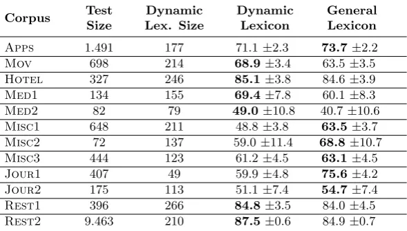
In order to evaluate the Dynamic Lexicons obtained for each domain, we separated 18% of each corpus (14.337 opinions, see Table 2) before building the respective DL. We apply a simple lexicon based heuristic for sentiment detection: we compute the sentiment of an opinion through the valence average of the affective words it contains (inverting the valence of negated words). For each domain, we compare the results obtained using the corresponding DL with the results obtained using a General Lexicon (GL) with word polarities for Spanish ((Saralegi and San Vicente, 2013), versionElhPolar esV1.lex has 5.200 words). In Table 3 we show the Macro-F measure for each corpus and for each lexicon (DL vs GL). This evaluation was carried out on the portion of the corpus reserved for testing.
As can be seen, for most specific domain corpora (movies, hotels, restaurants, medicine) the classifier based on the Dynamic Lexicon reaches slightly better results than the one based on the General Lexicon, except for apps domain. On the other hand, for corpora with opinions covering different domains (mis-cellaneous and journalistic texts) the General Lexicon has a better performance, as expected. The best performance was obtained using the domain specific lexicon on the largest corpus (REST2), reaching a Macro-F of 87.5
Corpus Test Size
Dynamic Lex. Size
Dynamic Lexicon
General Lexicon
Apps 1.491 177 71.1±2.3 73.7±2.2
Mov 698 214 68.9±3.4 63.5±3.5
Hotel 327 246 85.1±3.8 84.6±3.9
Med1 134 155 69.4±7.8 60.1±8.3
Med2 82 79 49.0±10.8 40.7±10.6
Misc1 648 211 48.8±3.8 63.5±3.7 Misc2 72 137 59.0±11.4 68.8±10.7 Misc3 444 123 61.2±4.5 63.1±4.5 Jour1 407 49 59.9±4.8 75.6±4.2 Jour2 175 113 51.1±7.4 54.7±7.4
Rest1 396 266 84.8±3.5 84.0±4.5
Rest2 9.463 210 87.5±0.6 84.9±0.7 Table 3: Macro-F1 for each corpus using the Dynamic Lexicons
and the 5.200 words General Lexicon.
(a)Rest2 (b)Med1
Figure 3: Word clouds results.
In Figure 3 we show some word clouds for restaurant and medicine domains. Bigger words represent higher valences, while green/red colors represent positive/negative words respectively. This graphical representation of the result helps to intuitively understand how well the Dynamic Lexicon behaves in the domain where it had been inferred. Note that words like ‘cerdo’ (‘pig’), that have a positive valence in the Restaurants domain, could have a negative valence in other cases.
5
Conclusions
We have presented a semi-supervised mechanism for building a sentiment lexicon from unlabeled corpora and a set of seed words (namedIL). The resources we have generated prove that it is possible to build a lexicon considering the words contexts as long as the corpus belongs to a specific domain. The generated lexicons achieve a competitive score in comparison to external general-purpose lexicons, even having much fewer words. Also, as it was expected, our sentiment lexicons induced from specific domains produced better results than those induced from general domain corpora, in which case a general-purpose lexicon works slightly better.
The context-graph proposal has value in itself. We have mentioned only one valence propagation mechanism but other algorithms over it could be applied. Also, the context-graph can be used for other problems in which the words context must be taken into account.
References
Azzinnari, A. and Mart´ınez, A. (2016). Representaci´on de palabras en espacios de vectores. Proyecto de grado, UdelaR (Universidad de la Rep´ublica).
Boldrini, E., Balahur, A., Martinez-Barco, P., and Montoyo, A. (2009). Emotiblog: an annotation scheme for emotion detection and analysis in non-traditional textual genres.Proceedings of the 1st Workshop on Opinion Mining and Sentiment Analysis, WOMSA09, pages 491–497.
Chen, Y. and Skiena, S. (2014). Building sentiment lexicons for all major languages. InProceedings of the 52nd Annual Meeting of the Association for Computational Linguistics (Volume 2: Short Papers), volume 2, pages 383–389.
Cruz Mata, F., Troyano Jim´enez, J. A., Enr´ıquez de Salamanca Ros, F., and Ortega Rodr´ıguez, F. J. (2008). Clasificaci´on de documentos basada en la opini´on: experimentos con un corpus de cr´ıticas de cine en espa˜nol. Procesamiento del lenguaje natural. N. 41.
Dubian, L. (2013a). Analisis de sentimientos sobre un corpus en espa˜nol: Experimentaci´on con un caso de estudio. Jornadas Argentinas de Inform´atica.
Dubian, L. (2013b). Procesamiento de lenguaje natural en sistemas de an´alisis de sentimientos. Tesis de grado, UBA (Universida de Buenos Aires).
Esuli, A. and Sebastiani, F. (2007). Pageranking wordnet synsets: An application to opinion mining. InProceedings of the 45th Annual Meeting of the Association for Computational Linguistics, pages 424–431. Association for Computational Linguistics.
Ghag, K. and Shah, K. (2014). SentiTFIDF sentiment classification using relative term frequency inverse document frequency. International Journal of Advanced Computer Science and Applica-tions(IJACSA), 5(2).
Hamilton, W. L., Clark, K., Leskovec, J., and Jurafsky, D. (2016). Inducing domain-specific sentiment lexicons from unlabeled corpora. CoRR, abs/1606.02820.
Hatzivassiloglou, V. and McKeown, K. R. (1997). Predicting the semantic orientation of adjectives. In Proceedings of the 35th Annual Meeting of the Association for Computational Linguistics and Eighth Conference of the European Chapter of the Association for Computational Linguistics, pages 174–181, Stroudsburg, PA, USA. Association for Computational Linguistics.
Jim´enez-Zafra, S. M., Mart´ın-Valdivia, M. T., Molina-Gonz´alez, M. D., and na L´opez, L. A. U. (2009). Corpus COAR, with opinions about restaurants. Available in: http://sinai.ujaen.es/coar/(last access 02/11/17).
Jim´enez-Zafra, S. M., Mart´ın-Valdivia, M. T., Molina-Gonz´alez, M. D., and Ure˜na L´opez, L. A. (2017). Corpus annotation for aspect based sentiment analysis in medical domain. International Artificial Intelligence in Medicine Conference (AIME).
Jurafsky, D. and Martin, J. H. (2017). Speech and Language Processing. (Book Draft), 3 edition.
Kamps, J., Marx, M., Mokken, R., and De Rijke, M. (2004). Using wordnet to measure semantic orientations of adjectives. Institute for Logic, Language and Computation (ILLC), FNWI.
Levin, B. (1991). Building a lexicon: The contribution of linguistics. International Journal of Lexicogra-phy, 4(3):205.
Liu, B. (2012). Sentiment Analysis and Opinion Mining. Morgan-Claypool.
Molina-Gonz´alez, M. D., Mart´ınez-C´amara, E., Mart´ın-Valdivia, M. T., and Urena-L´opez, L. A. (2014). Cross-domain sentiment analysis using spanish opinionated words. InInternational Conference on Applications of Natural Language to Data Bases/Information Systems, pages 214–219. Springer.
Mordecki, G., Kremer, F., and Dufort y Alvarez, G. (2015). Estudio de reputaci´on a partir de comentarios extra´ıdos de redes sociales. Proyecto de grado, UdelaR (Universidad de la Rep´ublica).
Mori, M., Tambucho, M., and Cardozo, D. (2016). Estudio de reputaci´on a partir de comentarios extra´ıdos de redes sociales. Proyecto de grado, UdelaR (Universidad de la Rep´ublica).
Muhammad, A., Wiratunga, N., Lothian, R., and Glassey, R. (2013). Contextual sentiment analysis in social media using high-coverage lexicon. InInternational Conference on Innovative Techniques and Applications of Artificial Intelligence, pages 79–93. Springer.
Pang, B. and Lee, L. (2008). Opinion mining and sentiment analysis. Foundations and Trends in Information Retrieval, 2:1–158.
Plaza-Del-Arco, F., Mart´ın-Valdivia, M., Zafra, S. M., Gonz´alez, M. D., and Mart´ınez-C´amara, E. (2016). Copos: Corpus of patient opinions in spanish. application of sentiment analysis techniques. SINAI Research Group, Universidad de Jaen, 57:83–90.
Polanyi, L. and Zaenen, A. (2006). Contextual valence shifters, chapter 1. computing attitude and affect in text: Theory and applications.
Ros´a, A., Chiruzzo, L., Etcheverry, M., and Castro, S. (2017). RETUYT in TASS 2017: Sentiment analysis for spanish tweets using SVM and CNN. InProceedings of TASS 2017: Workshop on Sen-timent Analysis at SEPLN co-located with 33nd SEPLN Conference, volume 1896. CEUR Workshop Proceedings.
Salvia, D. and Mechulam, N. (2018). Construcci´on de l´exicos din´amicos para el an´alisis de sentimientos. Proyecto de grado, UdelaR (Universidad de la Rep´ublica).
Santos, A. P., Oliveira, H. G., Ramos, C., and Marques, N. C. (2012). A bootstrapping algorithm for learning the polarity of words. In International Conference on Computational Processing of the Portuguese Language, pages 229–234. Springer.
Saralegi, X. and San Vicente, I. n. (2013). Elhuyar at tass 2013. InProceedings of XXIX Congreso de la Sociedad Espa˜nola de Procesamiento de Lenguaje Natural, Workshop on Sentiment Analysis at SEPLN (TASS2013).
Taboada, M., Brooke, J., Tofiloski, M., Voll, K., and Stede, M. (2011). Lexicon-based methods for sentiment analysis. Computational Linguistics, 37(2):267–307.
Turney, P. D. and Littman, M. L. (2002). Unsupervised learning of semantic orientation from a hundred-billion-word corpus. CoRR, cs.LG/0212012.
Vilares, D., Thelwall, M., and Alonso, M. A. (2015). The megaphone of the people? Spanish SentiStrength for real-time analysis of political tweets. J. Inf. Sci., 41(6):799–813.
6
Appendix
In this section we show some examples extracted from the corpora described in Table 1.
• Corpus APPS (Dubian, 2013b)- Rank: NEGATIVO - Compre un galaxy s3 ... Una estafa. Nunca responde el servicio de atencion al cliente. Compre un galaxy s3 que prometia 50gb durante 2 a˜nos y ha pasado ya un a˜no y pese a que reclame mil veces la respuesta nunca llego. Sansung y dropbox estafadores.
• Corpus MOV (Cruz Mata et al., 2008)- Rank: 1 - La alianza del mal. Resumen: Silicona, esteroides, pactos demon´ıacos y otras basuras habituales son la base que sustentan esta aberraci´on. De verguenza. Comentario: Una fiesta llena de excesos, rubias despampanantes, musculitos por doquier, alg´un que otro muerto. nada nuevo. La alianza del mal es el nombre de este Thriller sobrenatural que narra ... Porque la ´unica realidad es que La alianza del mal es un desecho cinematogr´afico, una insufrible sucesi´on de im´agenes cuya nica virtud es la de no durar demasiado. De vergenza.
• Corpus HOTEL (Molina-Gonz´alez et al., 2014)- Rank: 5 - Un hotel digno de menci´on! Como bien les coment´e a los propietarios a la hora de abandonar el hotel, no dudar´e un momento en recomendar una y otra vez el Hotel Albero de Granada. Su situaci´on respecto del centro de Granada no es la mejor, pero para nuestros prop´ositos era perfecto (escapada de fin de semana con visita a la Alhambra). Se encuentra en la carretera de paso a Sierra Nevada y muy cercano a la Alhambra. Por la zona se puede encontrar aparcamiento y este se encuentra en una zona segura y tranquila. Los parkings del centro de Granada que nos recomendaron en el hotel fueron lo que nos dijeron (nada caros) y pudimos movernos por el centro perfectamente desde all´ı. Las habitaciones muy limpias y las camas confortables. El desayuno fue espectacular. Ya ten´ıamos buenas referencias de este maravilloso hotel de una estrella (que para m´ı que viajo constantemente son m´as) pero ha superado con creces nuestras expectativas. Si vuelvo a Granada no dudar´e en hospedarme en el mismo hotel. Muchas gracias por todo!
• Corpus MED1 (Plaza-Del-Arco et al., 2016)- Rank: 5 - Todo un acierto. Encantado de ser su paciente. Siempre se toma su tiempo para saber tu caso y resolver tus dudas.
• Corpus MED2 (Jim´enez-Zafra et al., 2017)- Rank: NEGATIVE - En lugar de calmar el dolor por una infecci´on dental, me da efectos secundarios desagradables y una horrible migra˜na al d´ıa siguiente. El Tramadol 5 es mucho mejor.
• Corpus MISC1 (Vilares et al., 2015)- Rank: 4 - @Chunjiram @LjoeRam Son tan adorables, ajkjgshdkjhegftws.
• Corpus MISC2 (Mart´ı Anton´ın et al., 2016)- Rank: NEGATIVO - No lo he utilizado mucho.Actualmente (agosto 2002) tiene 22.800 km.Con solo 22.000, averia del embrague 70.000 ptas. Que dice Seat at.cliente? ha pasado la garantia no se hacen cargo,a pesar, que el mecanico me dijo que NO se debia a mal uso por mi parte. Lo arreglo. Resulta que el pedal, una vez arreglado, no sube del todo. Me lo vuelven a arreglar y actualmente sigue mal. Tiene ujnh ruido en los bajos que parece un concierto. No m atrevo a viajar.
• Corpus MISC3 (Mori et al., 2016)- Rank: POSITIVO - Uruguay se flore´o en casa y est´a un poco m´as cerca de Rusia 2018 https://t.co/mu5UJJL4P SOYCELESTE @SoyCelestee https://t.co/tt8bpbEP2y.
• Corpus JOUR1 (Mordecki et al., 2015)- Rank: NEGATIVO - anuncio de Batlle sobre juicio a ex socios del Comercial. Batlle dijo que cuando recuerda la conversaci´on con Mulford, del Credit Suisse, siente ”ganas de matar”.
• Corpus JOUR2 (Boldrini et al., 2009)- Rank: POSITIVE- Ahora vamos a lo nuestro, el tema del calentamiento global es uno de los m´as interesantes y conocer sobre el protocolo de Kyoto se hace sumamente necesario. Es por eso que en esta oportunidad les traigo un informe que publicaron los 147 amigos de la BBC Mundo que espero te sirva para conocer un poco m´as sobre esta situaci´on que a todos nos involucra.
• Corpus REST1 (Jim´enez-Zafra et al., 2009)- Rank: 1,3 - Caro para el conjunto ofrecido. Aunque los alimentos estaban bien cocinados no me pareci´o coherente el precio que se paga con lo ofrecido en general. Desde mi punto de vista, cuando pagas 45-50 persona hay muchas cosas que valorar y que deben ser coherentes con el precio: la forma de servir los platos, la cuberter´ıa, la manteler´ıa, etc. Todo debe ser coherente con esos precios y en este restaurante no lo es: manteles personales de pl´astico, vasos de tubo para refrescos, presentaci´on del producto anticuado, etc. Creo que pagar esos precio para el conjunto que ofrecen no es apropiado sino mas bien caro.