INTER-DISTRICT WATER ALLOCATION
WITH CONJUNCTIVE USE
James Roumasset
University of Hawaii
Rodney Smith
University of Minnesota
INTRODUCTION (Section 1)
The combination of increasing water scarcity and fiscal discipline has intensified the search for methods that increase the efficiency of water use. One method in particular that has received considerable attention in both theory and practice is the institution of interdistrict water trading. It is generally assumed that water trading can correct the inefficiencies of historically or politically determined water entitlements by equalizing the marginal value of water across districts.
We show in this paper that the simplifying assumptions under which water trading achieves efficient water allocation are rather severe. In a more realistic setting, a water authority is needed to establish rules and standards such that trading can achieve and sustain an efficient outcome.
In particular, we investigate the complicating role that space and time have on optimal water allocation rules. In a model where water transport is not costless, water at different locations have different values in the efficient solution. Similarly, when water storage is feasible but not costless (e.g. when groundwater is among the important sources of water) the spatial allocation problem is neither separable across periods nor does the intertemporal allocation problem have a simple and obvious solution. Finally, transportation cost functions may be non-linear in distance and volume: in addition, such functions might be discontinuous as well.
This paper discusses these complicating factors in a realistic setting involving two water districts on the Island of Oahu, Hawaii. The two districts are separated by a natural barrier but supplied by a common source. In addition to the shared source, one district has groundwater while the other has its own surface water supplies. Over time, the efficient solution involves changes in the allocation of the common water source.
In our example, the efficient allocation involves first allocating all of the common water to the groundwater district, then sharing the water between the two districts, and finally, allocating the common water to the surface water district. It is only when the common source is shared that the marginal valuation of water is equalized across the two districts, after allowance for transportation costs.
Section 2 below reviews the principles of efficient allocation over space and time. Section 3 provides principles for a more general model and applies them to the Hawaii case. Section 4 summarizes the primary principles for efficient inter-district allocation and provides concluding remarks regarding alternative institutions for approximating that solution.
EFFICIENT SPATIAL AND INTERTEMPORAL WATER ALLOCATION (Section 2)
Principles of Efficient Spatial Allocation (Section 2.1)
Suppose there is a single source of surface water (e.g. a diversion dam) and several users at different locations. The marginal cost of water at the headworks is just the cost of operating the facility to let an additional unit of water flow out (possibly negligible) plus the user cost (rent plus interest plus depreciation) of the additional headworks capacity needed for that marginal unit. Efficient water allocation to a user adjacent to the headworks requires that this marginal cost of water equal the marginal benefit to the user. If the user is a farmer, for example, the marginal benefit is the value of the additional product that the marginal unit of water provides.
to transport the marginal unit of water plus the value of water lost in conveyance (e.g. through evaporation, seepage, and percolation). Ideally, conveyance structures are designed to minimize transportation costs such that the marginal cost of reducing conveyance losses by one unit is equal to the marginal benefit of the water thus saved. In summary, efficient allocation requires setting the net marginal benefit at each location in the water distribution system, after deducting the marginal transportation cost, to the marginal cost of providing water at the headworks of the system.1
We define the marginal cost at the headworks as the “system efficiency price” and the gross marginal benefit (before deducting transport costs) as the locational efficiency price. The efficiency conditions stated above imply that the locational efficiency prices differ by the transportation cost between locations and that the system efficiency price is the locational efficiency price at the headworks.
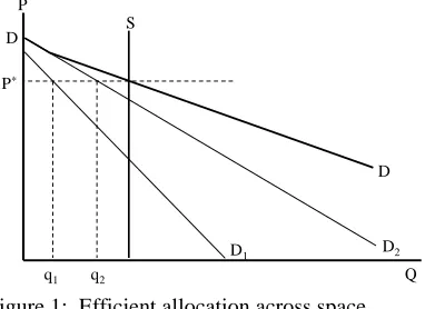
Figure 1 illustrates optimal allocation of surface water for two sub-districts. One sub-district is at the headworks and requires no transportation costs. The other is more distant with commensurate costs. Curves D1 and D2 are the net water demand curves for
sub-districts 1 and 2 after deducting transport costs. The curve DD is the combined demand of the two sub-districts and S is the (inelastic) supply of surface water. The efficiency price is P*, where the combined demand curve intersects the total supply curve S. Here, q1 and
q2 give the optimal allocation for each respective
subdistrict, and are the levels at which the respective inverse demand in each subdistrict is equal to the price P*.
P
S
D1 D2
D
D P*
Q q1 q2
Figure 1: Efficient allocation across space
There are a number of institutional mechanisms for achieving, or at least approximating, efficient allocation. To the extent that information about marginal benefits is decentralized, decentralized mechanisms of water allocation, especially water pricing and water trading,
are thought to be preferable to centralized mechanisms such as water rationing. Water pricing will achieve efficient allocation if the marginal price for each user is set equal to the locational efficiency price at the user’s location. Intramarginal prices need not be so set. For example, the water authority may attain both efficiency and equity through block pricing, the simplest form of which is to charge nothing for an amount judged to be a necessity2 and the locational efficiency price for all subsequent units. This simple pricing scheme achieves both efficiency and progressivity in the sense that the average price increases with the amount of water consumed.
If there are substantial non-linearities in production and transport costs, however, then marginal costs are dependent on the quantities consumed, which the water authority may not be able to accurately estimate without knowing the marginal benefit schedules for its (possibly diverse) clientele. This problem may be largely overcome over time, through a combination of estimation and observation of quantities consumed.
A less informationally-demanding institution is water trading. The water authority approximates entitlements consistent with efficiency and equity. Trading then restores efficiency without decreasing equity. But since water at different locations is not equally valuable, the authority needs to set appropriate trading rules and standards. Suppose, for example, that water is conveyed in pipes and that leakage is negligible. In that case, trading can be conducted on a one-for-one basis across different locations, and water users can be required to pay for transport costs in addition to what they pay for the water entitlement itself. To take the other polar extreme, suppose that transport costs consist entirely of conveyance losses. In this case, trading can be conducted in terms of “gross” water (i.e. water at the headworks). Users are then entitled to receive their allocated amount of gross water minus the conveyance losses involved. Alternatively, trading can be conducted in terms of water received but the authority establishes exchange rates that achieve the same result. In general, if either or both types of transport costs are present, the authority can set exchange rates as given by the ratios of appropriate locational efficiency prices.
Principles of Efficient Intertemporal Allocation: the Case of Groundwater (Section 2.2)
in present value associated with extracting a unit of water now instead of later. One such loss is the decrease in present value from forgoing the capital gains that would have accrued from conserving the unit. The other is the loss in present value from having to extract water from deeper in the well.
A major source of Honolulu water supply is the Pearl Harbor Aquifer. In that case the marginal user cost is roughly four times the marginal extraction cost (i.e. the full marginal cost or system efficiency price is five times the marginal extraction cost).3
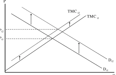
In Figure 2, demand increases from Dt1 in period 1 to
Dt2 in period 2, and total marginal cost increases from
TMCt1 in period 1 to TMCt2 in period 2. Figure 2
illustrates optimal extraction from a groundwater source in two periods. Because of the upward (but not vertical) slope of the total marginal cost curve and because of the tendency of demand to increase more than the total marginal cost from one period to the next, the efficiency
price may increase less than in the surface water case. This tendency plays an important role in the Hawaii simulations to follow.
Figure 2: Efficient allocation across time
In a case like that depicted in Figure 2, water trading can be rendered efficient by allowing forward contracting. This is equivalent to setting exchange rates for water in different periods according to the ratio of efficiency prices (full marginal costs) across periods.
Conjunctive Use With Spatially-Equivalent Sources (Section 2.3)
Now suppose that a water district has two locationally equivalent sources – one surface water source and one groundwater source. The efficiency conditions are just those of section 2.1 with the additional condition that the full marginal cost of providing water from both
sources is equal. This case readily generalizes to more than two sources.
Unrestricted Interdistrict Allocation (Section 2.4)
Next consider the case of two districts, each with its own source. To illustrate the principles involved and to facilitate the transition to the Hawaii application, we assume that district 1 is sourced by groundwater and that district 2 is sourced by surface water. Intradistrict transport costs are assumed to be zero.
Figure 3 illustrates the optimal allocation for two sub-cases. The water demand curve in district 1 is labeled D1 and the demand curve in district 2 is labeled D2.
Likewise, the respective total marginal cost (TMC) curves, or supply, for each district are labeled S1 and S2.
In the first sub-case, interdistrict transport costs are prohibitively expensive. In such a case the optimal solution is given by the intersection of each district’s demand curve with its own TMC curve. Note that efficiency price (at the intersection point) in district 1 is higher than that of district 2, although this may change if the demand for water is growing.
For the second subcase, assume that interdistrict transport costs are zero. Total demand DD is given by the horizontal sum of district 1 and district 2 demand curves. Total marginal cost, or supply, is given by the sum of groundwater S1 and surface water S2 supplies
from the two districts, and is represented by ST. In the case shown, S2 – q2 units of water are shipped from
district 2 to district 1 in order to achieve the requirement that the efficiency prices be equal (to P*) in both districts.
P
S2
Q D
D ST
D2 D1
P*
q2 q1
S1
Figure 3: Efficient conjunctive use without conveyance costs
Dt2
Dt1
Pt2
Pt1
TMC t1
TMCt2
Towards a More General Model of Efficient Intertemporal and Spatial Allocation (Section 3)
Spatial equivalence among sources facilitates a relatively simple solution. In effect, one can subtract the fixed quantity of surface water from demand, unify the various groundwater sources according the principle of equalizing the full marginal cost across wells, and then solve the problem as if there is a single groundwater source. When spatial equivalence does not hold (i.e. when sources are at different locations) we lose this separability between supply and demand. Moreover, there is no reason to expect that water be fungible across the entire system. Rather, the optimal solution is likely to exhibit spatial separability between districts, where different districts have different system efficiency prices. However, the boundaries of these districts are in general unknowable without doing the optimization exercise.
The Hawaii example discussed in this section illustrates some of the complexities that can arise. Our discussion is framed in the more general water allocation problem described in the introduction. A water authority manages water for two districts (sources of demand) and has four water sources. Demand in each district grows over time, possibly at different rates. Each district has its own source of water and they can share a third source. The first district has rechargeable groundwater while the other district has surface water. The shared source is surface water. The fourth source comes from desalination, which serves as a backstop technology. Desalination is used only when the system efficiency price of water in a district rises to the desalination cost.
Efficient allocation now requires interdistrict efficiency as well as intradistrict efficiency. The latter requires that the marginal benefit at each location and at each time be equal to the locational efficiency price at the corresponding time. Interdistrict efficiency in a particular period requires either that the system efficiency prices are equal across districts or that the prices are different and that all of the common source water is allocated to the higher-priced district (See Smith and Roumasset 1999). Solving for the optimal solution in this case is not obvious. One cannot, for example, choose an allocation of common source water, solve for the intradistrict optimal use of water then iterate on the original allocation according to which district has the higher efficiency price. In general, the optimal allocation of common source water will itself change over time.
Assuming equal and constant marginal water transport costs, the optimal solution for the Oahu case is illustrated in Figures 4 and 5. Figure 4 shows the
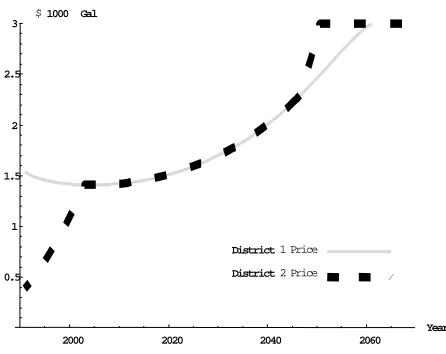
optimal sharing rule for the common water source, and Figure 5 shows the optimal water pricing rule for water in each district over time. For the first eight years, the full cost of producing water from the groundwater district is so much higher than the surface water district that even allocating all of the aqueduct water to the former leaves the system efficiency price of district 1 higher than that of district 2. But the growth of demand in the face of an inelastic supply causes the system efficiency price in district two to rise faster than that in district one (see Figure 5). Eventually, water prices in the two districts are equal and some of
Figure 4. Declining share of common-source water allocated to the groundwater district
the common source water is allocated to the second district. The amount of the shared resource received by the second district increases until eventually it receives all of the shared water. Once the second district receives the entire amount of the shared source, water prices then begin to diverge, with district two prices higher than district one prices. This process continues until both sides adopt the backstop technology.
FJZYK40D.wmf
2000 2020 2040 2060
Year 0.5
1 1.5 2 2.5 3
$1000 Gal
District 1 Price District 2 Price
Figure 5. Efficiency prices over time
2000 2010 2020 2030 2040 2050 2060
Year 5000
10000 15000 20000 25000
Si
This example shows the potential problem inherent in sharing rules that are constant over time (e.g., deciding each district gets half of the shared water source each year). This is especially true if the districts are not allowed to trade their water allocations.
The solution described in Figures 4 and 5 can be implemented by water prices or by trading. In the case of pricing, a central water authority is needed to establish pricing schedules (e.g. block pricing) that conform to the time-denoted locational efficiency prices established in the optimal solution. Alternatively, the central authority can facilitate the same solution via trading by extending the locational exchange rates discussed in section 2.1 to inter-district trades. Under conditions of full information, the two mechanisms will achieve the same allocation. Trading has the usual advantage under conditions of imperfect information in that the market can correct mistakes in the initial allocation. Suppose, for example, that the Water Commission allocates the aqueduct water to the two districts on a 50-50 basis, regardless of the year. This will result in district 1buying water rights from district 2 before 2021 and vice versa from 2022 on.
Summary and Concluding Remarks (Section 4)
The central principle for efficient allocation of water over space is to take water from the abundant district and give it to the scarce district until the scarcity values or efficiency prices are equalized. Where water is fungible over time, as in the case of groundwater or conjunctive use, water should be conserved to that extent which maximizes the present value of the water resources. That implies that the efficiency price should be allowed to rise, albeit somewhat slower than the prevailing interest rate. Where intra and inter-district costs of conveyance are significant, these should be deducted from the gross marginal benefits of water.
Section 3 illustrated the case of asymmetrical transport costs with quantity restrictions. In this case, the efficient solution may involve an internal optimum, such that efficiency prices are equal across districts; or a “corner solution,” such that the districts are managed independently, one with efficiency prices than the other.
Note that the interdistrict efficiency conditions require that the district-level conditions are also being satisfied. For example, the principle of equalizing efficiency prices across districts (where feasible) requires that mechanisms for achieving intradistrict efficiency regarding spatial allocation and conjunctive use are in place.
As a final caveat, note that despite the prominence of “efficiency prices” in the forgoing discussion, all of the allocation rules refer to quantities of water. Actual prices are not required in the mechanism chosen to implement the efficiency rules. It is imaginable that water quantities could be centrally chosen so as to achieve the requisite equalities of efficiency prices without ever having used prices in practice. Whether or not this is advisable, depends on how knowledgeable a central water authority may be regarding the idiosyncratic benefits of individual users. But even the commitment to a decentralized mechanism does not require charging everyone the marginal cost of water for every unit of water used. As discussed in the various sections above, other mechanisms such as block pricing and water trading can also be used to achieve the efficient quantity allocations.
But none of these institutional mechanisms, however “market-based,” is capable of implementing the efficient solution without actually exercising an algorithm such as the one described here. A unit of water in one time period and at one location is not identical to that in another and cannot be traded as such. In order to facilitate efficient water trading, a water authority is still needed to establish exchange rates that create equivalencies between units of water in different times and different places according to the minimum cost of transporting water across space and the financial opportunity cost of “transporting” water across time. In some cases, these exchange rates are independent and can be announced a priori. In other cases, the exchange rates themselves depend on the optimal solution, necessitating the simulation exercise before the rates can be announced.
REFERENCES
Chakravorty, U. and J. Roumassset. 1991. “Efficient Spatial Allocation of Irrigation Water.” American
Journal of Agricultural Economics. 73:165-73.
Chakravorty, U., E. Hochman, and D. Zilberman. 1995. “A Spatial Model of Water Conveyance.” Journal of
Environmental Economics and Management.
28:25-41.
Krulce, D., J. Roumasset, and T. Wilson. 1997. “Optimal Management of a Renewable and Replaceable Resource: The Case of Coastal Groundwater.” American Journal of Agricultural
Economics. 79:1218-1228.
Smith, R.B.W., and J. Roumasset. 1999. “Constrained Conjunctive-Use for Endogenously Separable Water Markets: Managing the Waihole-Waikane Aqueduct.” WP no. 00-6, Dept. of Economics, U. of Hawaii.
ENDNOTES
1 See e.g. Chakravorty and Roumasset (1988) and
Chakravorty et. al. (1995) for formalizations of this problem.
2
For example, 160 gallons per day per household of four persons.
3 See Krulce et. al. (1997) for the formal model and an