93
Comprehensive Review on Shortest Path
Algorithms in Networks
Meenakshi
ABSTRACT
In this paper the shortest-path problem in networks is considered in which the delay (or weight) of the edges changes with time acc or ding to arbitrary functions. The author studied algorithms for finding the shortest-path and minimum delay under various waiting constraints and investigate the proper ties of the derived path. We show that if departure time from the source node is unrestricted then a shortest path ca n be found that is simple and achieves a delay as short as the most unrestricted path. I n the case of restricted transit, it is shown that there exist cases where the minimum delay is finite but the path that achieves i t is infinite.
Keywords: shortest path, algorithms, genetic, WSN, network.
1. INTRODUCTION
Shortest paths algorithms have been the subject of extensive research for many years resulting in a large number of algorithms for various conditions and constraints. The vast majority of these deal with fixed graphs i.e., fixed topology and fixed link weights. The advancement of computer networks and distributed processing has brought renewed interest in the subject with a new twist: time dependency. Several works have been published dealing with topological change s in which links may occasionally become unavailable (i.e., infinite weight) and others deal with quasi static models, that is, link weights that change from time to time but remain constant in between these (infrequent) change. Time dependent shortest path problems have been studied for the ca se of discrete delay functions whose domain and range are the positive integers. Such problems were addressed both directly [4,5] and indirectly in the context of maximal flow[6,7]. In this paper we address the shortest path problem without these restrictions, i.e., we allow arbitrary functions for link delays. In this respect this is the broadest generalization. Such a problem was briefly treated by Dreyfus and Ling et.al.[9] which address only limited case s.
The most direct treatment to date was done by Halpern where arbitrary waiting times are also consider ed. In this latter work an algorithm is proposed for various waiting constraints, but this algorithm cannot be bounded by network topology (i.e., the number of operations cannot be bounded by a function of the number of nodes or edge s) nor are the proper ties of the resulting path investigated (e.g., whether it is a simple path). All the above works avoid the treatment of functions by addressing the problem for a single instance of time and not for time range s. In this paper we present algorithms for finding the shortest-path and minimum-delay for all instances of time and under various waiting constraints and investigate proper ties of the derive d path. We show that if message s ca n be arbitrarily delayed at the source node then a shortest path ca n be found that is simple and achieves a delay as short as the most unrestricted path, without having to waitenroute.
Our interpretation of time dependency of links is that of message traversal. For example, one interpretation might be the delay incurred by a message traversing the links. We note that time dependency may not be a continuous function. Consider a dial-up link between two nodes which is established and disestablished periodically. A message arriving while the link is established will suffer a relatively short delay while a message arriving immediately after the link is disestablished will suffer a much greater delay. We also do not restrict ourselves to FIFO links only, since in some potential cases the FIFO assumption is invalid. For example, consider a link composed of two physical communication channels one being faster than the other. If the policy of link management is to send a message over the first available channel, then a message sent over the slower one may arrive later than another message, sent later on the faster channel, meaning that message s arrive in a non-FIFO order
94 wondering whether to take the local train stopping in front of him or to wait for the express train to his destination. Here again, we have time dependency of delays, with possible non-FIFO behavior.
General Networks
In this part, we focused on the problem of maintaining the shortest-path tree from a given source of a general graph with positive real edge weights, whose topology undergoes dynamic changes. This problem has been widely studied both theoretically and experimentally. From the theoretical point of view, some solutions have been proposed. Some of them are only able to cope with the update of one edge at a time while others can handle also batch updates up dates that consist of multiple edge changes at a time. To the best of our knowledge, none of the above solutions is asymptotically better than recomposing the shortest paths from scratch, by applying Dijkstra’s algorithm in the worst case. From the experimental point of view, very few studies are known. The most recent is that in an experimental evaluation of the algorithms in and some of their variants for batch updates. The most important conclusion of this paper is the astonishing level of data dependency within the problem.
The second outcome is that it is useful to process a set of updates as a batch when updated edges have strong interference w. r. t. their impact on the shortest-path tree. While updates that are far away from each other usually do not interfere, and hence they can be handled iteratively. Our contribution to this area is the following: we have developed two new dynamic algorithms for homogeneous batches either incremental (containing only insert and weight decrease operations) or detrimental (containing only delete and weight increase operations) batches which model realistic dynamic scenarios like node failures in communication networks. We have showed that they extend the results of to general graphs, and to batch updates, and those of to batch updates. We have proved the new algorithms to be theoretically efficient in case of homogeneous batches. We have also provided an extensive experimental study that compares the new solutions with the most effective known batch algorithms. Our data show that the proposed algorithms improve over the literature in a set of realistic scenarios. Our results complement previous studies and show that the various solutions can be consistently ranked on the basis of the type of homogeneous batch and of the underlying network.
LEACH ALGORITHM FOR WSN
Heinzelman, et.al introduced a hierarchical clustering algorithm for sensor networks, called Low Energy Adaptive Clustering Hierarchy (LEACH). LEACH arranges the nodes in the network into small clusters and chooses one of them as the cluster-head. Node senses its target and then sends the relevant information to its cluster-head. Then the cluster head aggregates and compresses the information received from all the nodes and sends it to the base station. The nodes chosen as the cluster head drain out more energy as compared to the other nodes as it is required to send data to the base station which may be far located. Hence LEACH uses random rotation of the nodes required to be the cluster- heads to evenly distribute energy consumption in the network. TDMA/CDMA MAC is used to reduce inter- cluster and intra-cluster collisions. This protocol is used were a constant monitoring by the sensor nodes are required as data collection is centralized (at the base station) and is performed periodically .As shown in figure 1 below.
95 Simulation results of LEACH Algorithm for WSN shows that Number of packet sent to base station with each round and number of dead nodes form every round where dead nodes are absorbing whole data information before reaching to base station. Also with increasing number of nodes i.e. as the number of nodes pass 1500 energy dissipation in each round also increasing which become as the drawback of LEACH Algorithm.
Figure 2. Number of packets sent to Base Station Vs Rounds
Dijkstra’s Algorithm: Explanation and Implementation For each vertex within a graph we assign a label that determines the minimal length from the starting point s to other vertices v of the graph. In a computer we can do it by declaring an array d. The algorithm works sequentially, and in each step it tries to decrease the value of the label of the vertices. The algorithm stops when all vertices have been visited. The label at the starting point s is equal to zero (d[s]=0); however , labels in other vertices v are equal to infinity (d[v]=∞), which means that the length from the starting point s to other vertices is unknown. In a computer we can just use a very big number in order to represent infinity. In addition, for each vertex v we have to identify whether it has been visited or not.
In order to do that, we declare an array of Boolean type called u[v], where initially, all vertices are assigned as unvisited (u[v] = false). The Dijkstra’s algorithm consists of n iterations. If all vertices have been visited, then the algorithm finishes; otherwise, from the list of unvisited vertices we have to choose the vertex which has the minimum (smallest) value at its label (At the beginning, we will choose a starting point s). After that, we will consider all neighbors of this vertex (Neighbors of a vertex are those vertices that have common edges with the initial vertex). For each unvisited neighbor we will consider a new length, which is equal to the sum of the label’s value at the initial vertex v (d[v]) and the length of edge l that connects them. If the resulting value is less than the value at the label, then we have to change the value in that label with the newly obtained value.
d [ neighbors ] = min ( d [ neighbors ] , d[ v ] + l ) (1)
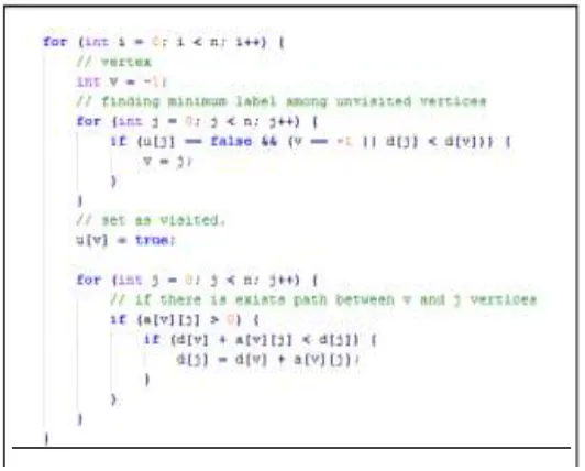
After considering all of the neighbors, we will assign the initial vertex as visited (u[v] = true). After repeating this step n times, all vertices of the graph will be visited and the algorithm finishes or terminates. The vertices that are not connected with the starting point will remain by being assigned to infinity. In order to restore the shortest path from the starting point to other vertices, we need to identify array p, where for each vertex, where v ≠ s, we will store the number of vertex p[v], which penultimate vertices in the shortest path. In other words, a complete path from s to v is equal to the following statement
96 Fig. 3: Implementation in Java: An Excerpt
Floyd-Warshall Algorithm:
Explanation and Implementation Consider the graph G, where vertices were numbered from 1 to n. The notation dijk means the shortest path from i to j, which also passes through vertex k. Obviously if there is exists edge between vertices i and j it will be equal to dij0, otherwise it can assigned as infinity. However, for other values of dijk there can be two choices: (1) If the shortest path from i to j does not pass through the vertex k then value of dijk will be equal to dijk- 1. (2) If the shortest path from i to j passes through the vertex k then first it goes from i to k, after that goes from k to j. In this case the value of dijk will be equal to dikk-1 + dkjk-1. And in order to determine the shortest path we just need to find the minimum of these two statements :
dij0 = the length of edge between vertices i and j (3)
dijk = min (dijk-1, dikk-1 + dkjk-1) (4)
97 Genetic Algorithm (GA)
Intelligent algorithms have been introduced in finding optimal shortest paths in many situations that require the systems to search through a very large search space within limited time frame and also in accommodating an ever-changing environment. One of these algorithms is GA. By definition, genetic algorithms are a class or group of ―stochastic search algorithms‖ that are based on biological evolution [8]. GA is mostly used for optimization problems. It uses several genetic operations such as selection, crossover, and mutation in order to generate a new generation of population, which represents a set of solutions (chromosomes) to the current problem. In addition, on average, this new generation is supposed to be better in terms of their overall fitness value as compared to the previous population. Each individual or chromosome within the population will be assigned a fitness value, which is calculated based on a pre-determined fitness function that measures how optimal its solution is in solving the current problem.
In order to solve the shortest path problem using the GA [9], we need to generate a number of solutions, and then choose the most optimal one among the provided set of possible solutions. In order to solve the problem, an initial population that forms the first set of chromosomes to be used in the GA is randomly created. Each chromosome represents one possible solution to the current problem at hand. After that, they (chromosomes) are estimated using certain fitness function, which determines how well the solutions are. Taking into account the fitness value of each solution or chromosome, some chromosomes or individuals will be selected (selection operation), and the basic genetic operations such as crossover and mutation are applied on these chromosomes. Then, the fitness value of each chromosome is re-calculated, and the best solutions are selected to be considered for the next generation. This process continues until the criteria of the given problem will not be achieved. Thus we can identify the following stages of a GA:
Step 1: Determine the fitness function; in our case we need to maximize the following function f(Chk) = (∑edge)- 1, where Chk is k-th chromosome and ∑edge is the sum of edges from starting point to final destination.
Step 2: Create initial population – a population that contains n individuals. At this stage we do not need to create fittest individuals, because it is probable that GA will transfer them into viable population. In order to create chromosomes for initial population, we will produce random paths from the starting point to final destination.
Step 3: Selection – the stage of GA that is used to select two chromosomes for genetic operations such as crossover and mutation. There are different types of selection methods; however, the Roulette Wheel selection method is chosen in order to solve the shortest path problem.
Step 4: Crossover – the process of reproduction where descendants are inherit traits of both parents mixing them in some way. Individuals for reproduction will be chosen from whole population (not from the survivors in the first iteration), because we need to keep diversity of individuals, otherwise entire population will be hammered with single copies of one individual. There exist different types of crossover methods; however, for our problem we will use the simplest method, which is called single point crossover.
Step 5: Mutation – the act of changing the value of some gene. Mutation keeps the genetic diversity of the population by changing genes of selected chromosome.
98 CONCLUSION AND FUTURE WORK
The computed time complexity for each of the Dijkstra’s, Floyd-Warshall and Bellman-Ford algorithms show that these algorithms are acceptable in terms of their overall performance in solving the shortest path problem. All of these algorithms produce only one solution. However, the main advantage of GA over these algorithms is that it may produce a number of different optimal solutions since the result can differ every time the GA is executed. In the future, the proposed GA framework will be extended and improved in finding the shortest path or distance between two places in a map that represents any types of networks. In addition, other artificial intelligence techniques such as fuzzy logic and neural networks can also be implemented in improving existing shortest path algorithms in order to make them more intelligent and more efficient.
REFERENCES
[1]. S. Skiena, A. Revilla, ―Programming Challenges, The Programming Contest Training Manual‖ pp. 248 – 250.
[2]. S. Hougardy, The Floyd-Warshall, ―Algorithm on Graphs with Negative Cycles‖, University of Bonn, 2010.
[3]. M. Negnevitsky, Artificial Intelligence: A Guide to Intelligent Systems, Third Edition, Addison-Wesley, 2011.
[4]. I. Rakip, U. Atila, ―A Genetic Algorithm Approach for Finding the Shortest Driving Time on Mobile Devices‖, Scientific
Research and Essays, Dept. of Computer Engineering, 2011.
[5]. Dijkstra’s Algorithm, Available at http://informatics.mccme.ru/moodle/mod/statements/ view.php?id=193#1. 2012.
[6]. Floyd-Warshall Algorithm, Available at http://informatics.mccme.ru/moodle/mod/statements/ view.php?id=218#1. 2012.
[7]. Bellman-Ford Algorithm, Available at http://informatics.mccme.ru/moodle/mod/statements/ view.php?id=260#1. 2012.
[8]. Ford LR, Fulkerson DR. Flows in networks. Princeton, NJ: Princeton University Press; 1962.
[9]. Bellman RE. On a routing problem. Quarterly of Applied Mathematics 1958;16:87–90.
[10]. Pape U. Implementation and efficiency of moore algorithms for the shortest root problem. Mathematical Programming
1974;7:212–22.
[11]. Glover F, Klinkgman D, Philips N. A new Polynomial bounded shortest path algorithm. Operations Research 1985;33: 65–73.
[12]. Gallo G, Pallottino S. Shortest path methods. In: Florian M, editor. Transportation planning models. Amsterdam: Elsevier Science
Publishers; 1984. p. 227–56.
[13]. Hung SM, Divoky JJ. A computational study of efficient shortest path algorithms. Computers and Operations Research
1988;15(6):567–76.
[14]. VurenVT, Jansen GRM. Recent developments in path finding algorithms: a review. Transportation Planning and Technology
1988;12:57–71.
[15]. Cherkassky BV, Goldberg AV, Radzik T. Shortest paths algorithms: theory and experimental evaluation. Mathematical