_______________
E-mail address: [email protected] Received August 15, 2019
J. Math. Comput. Sci. 10 (2020), No. 1, 40-50 https://doi.org/10.28919/jmcs/4263
ISSN: 1927-5307
A NEW MONOTONICALLY STABLE DISCRETE MODEL FOR THE
SOLUTION OF DIFFERENTIAL EQUATIONS EMANATING FROM THE
EVAPORATING RAINDROP
OBAYOMI A. ADESOJI
Department of Mathematics, Ekiti State University, Ado-Ekiti, Nigeria
Copyright © 2020 the author(s). This is an open access article distributed under the Creative Commons Attribution License, which permits unrestricted use, distribution, and reproduction in any medium, provided the original work is properly cited.
Abstract. Most of the models of the dynamics of evaporating raindrop have been created using Ordinary Differential Equations. Some models assumed that evaporation is affected by air resistance that is negligible and proportional to the velocity of transition others assumed that the air resistance is significant and proportional to the square of the velocity. Because of the significant differences in the basic assumption used by various modelers, the solution of the resulting equations produced differed values There are yet no work to confirm these dependencies. In this work we obtain a class of hybrid finite difference schemes that can be used to obtain a reliable approximate solution to some of these differential equation models. The schemes were found to possess the same monotonic properties as the analytic solution.
Keywords: monotonically stable discrete model; differential equations emanating from the evaporating raindrop; hybrid finite difference schemes.
2010 AMS Subject Classification: 34C60, 34K60.
1.0 INTRODUCTION
An equation of state is a representation of a dynamic system as a function of state variables such
as pressure, temperature, volume and number of particles which are used to measure the status of
such system under a given set of physical conditions that may have effect on the measured
Evaporation is a type of vaporization of a liquid that occurs from the surface of a liquid into a
gaseous phase that is not saturated with the evaporating substance. Evaporation happens when
atoms or molecules escape from the liquid and turn into a vapor. Factors that may affect the way
and the rate at which evaporation occurs include: Saturation of the air, humidity, air pressure
and temperature of the liquid. The shape of a raindrop depends upon its size and the amount of
air resistance present during it drops. Some are round, others appear flattened at the bottom, and
then there are those that resemble jellybeans. For the purpose of this study, all the raindrops will
be considered as spheres. (see [3, 7]).
Most existing mathematical models of this dynamical system were developed based on the
principle of Newton’s law of motion. Each of these models considered two major variations.
Either that the raindrops are small particle bodies that is affected by air resistance significantly or
that the raindrops are big particles that floats through the air vacuums with insignificant air
resistance (see [6, 8]). Generally when a body in motion is treated as a particle rotational effects
are unimportant (or negligible), and also when the size of the object is negligible relative to the
scale of the system, only translational motion is relevant.
2.0 MATERIALS AND METHODS
The following ordinary differential equations have been considered while deriving a hybrid finite
difference scheme that can simulation the dynamics of the motion of an evaporating raindrop.
2.1 Model I [6]
These authors came-up with the Ordinary Differential Equation given below
𝑑𝑣 𝑑𝑡+
3(𝑘𝜌)
𝑡(𝜌𝑘)+𝑟0 𝑣 = 𝑔
(1)
ρ is the density of rainwater
𝑟0 is the initial radius of the raindrop
𝑟 =𝜌𝑘𝑡 + 𝑟0 is the radius of the raindrop at time t, k is a constant
𝑔 is acceleration due to gravity
2.2 Model II [6]
If we consider the small object theory we can arrive at the following model for the evaporating
𝐹 = 𝑚𝑑𝑣𝑑𝑡 = 𝑚𝑔 − 𝑘𝑣 (5)
Which gives a solution of the form
𝑣 =𝑚𝑔𝑘 (1 − 𝑒−𝑚𝑘𝑡 ) (6)
We will use a combination of interpolation and Nonstandard methods
3.0DERIVATION OF THE SIMULATION MODEL
To obtain a simulation model which can accommodate the assumption on air resistance and the
decay thru evaporation. We assume raindrop water has a density of 0.99823 grams/cubic
centimeter and a temperature of 4oC degrees Celsius. The water is evaporating with a speed proportional to the surface area. We are suggesting a new simulation model with the following
components.
y = a0+ a1x − a0𝛽𝑔
(𝛼𝑥+𝛽)3 + 𝑒−αx (7)
a0 is a known and measurable constant, 𝛼 and 𝛽 are simulation parameters. This interpolation
function will be used to derive a finite difference scheme for solution of first order Ordinary
Differential Equation. To get the hybrid scheme, we will apply nonstandard method to the step
size by replacing it with a normalized function (Obayomi&Oke2003). For the scheme:
Differentiating (7)
y′=a
1+ 3a0𝛼𝛽𝑔(𝛼𝑥 + 𝛽)−4+(− α)𝑒−αx (8)
y′=a
0(1 + 3(𝛼𝑥 + 𝛽)−4𝛼+(− α)𝑒−αx (9)
y′′ = −12a
0 α2𝛽𝑔(𝛼𝑥 + 𝛽)−5+ α2𝑒−αx (10)
y′′′= 60a
0α3(𝛼𝑥 + 𝛽)−6− α3𝑒−αx (11)
a0 = y
′′− α2𝑒−αx
(−12 α2𝛽𝑔(𝛼𝑥+𝛽)−5) (12)
or
a0 = y
′′′+α3𝑒−αx
(60α3(𝛼𝑥+𝛽)−6) (13)
a1 = y′+ α𝑒−αx - (𝛼𝑥+𝛽)α
2𝑒−αx 4α +
(𝛼𝑥+𝛽)y′′
4α (14)
3.1 Generation of the Finite Difference Model
y𝑛 = a0+ a1𝑥𝑛 − (𝛼𝑥𝑎0𝛽𝑔
𝑛+𝛽)3 + a0𝑒
−α𝑥𝑛 (15)
y𝑛+1 = a0+ a1𝑥𝑛+1 − (𝛼𝑥𝑎0𝛽𝑔
𝑛+1+𝛽)3 + a0𝑒
−α𝑥𝑛+1 (16)
y𝑛+1− y𝑛 =
= a1[(𝑥𝑛+1− 𝑥𝑛)+ 𝑎0𝛽𝑔{(𝛼𝑥𝑛+1+ 𝛽)−3− (𝛼𝑥𝑛+1+ 𝛽)−3} +a0(𝑒−𝛼𝑥𝑛+1− 𝑒−𝛼𝑥𝑛)] (17)
Let 𝑥𝑛 = a + nh 𝑥𝑛+1 = a + (n + 1)h
𝑥𝑛+1− 𝑥𝑛 = h (18)
Putting (17) in (18), we have
y𝑛+1 − y𝑛 = a1h +𝑎0𝛽𝑔{(𝛼[𝑎 + (𝑛 + 1)ℎ] + 𝛽)−3− (𝛼[𝑎 + 𝑛ℎ] + 𝛽)−3} +
(𝑒−𝛼(𝑎+𝑛ℎ){𝑒−𝛼ℎ− 1}) (19)
M = {(𝛼[𝑎 + (𝑛 + 1)ℎ] + 𝛽)−3− (𝛼[𝑎 + 𝑛ℎ] + 𝛽)−3}
N = (𝑒−𝛼(𝑎+𝑛ℎ){𝑒−𝛼ℎ− 1})
y𝑛+1 = y𝑛+ a1h +𝑎0𝛽𝑔M + N (20)
a0 = y
′′− α2𝑒−αx
(−12 α2𝛽𝑔(𝛼𝑥+𝛽)−5)
a1 = y′+ α𝑒−αx - (𝛼𝑥+𝛽)α 2𝑒−αx 4α +
(𝛼𝑥+𝛽)y′′
4α
y𝑛+1 = y𝑛+ hy′+ ℎα𝑒−αx (1 - 𝛼(𝛼𝑥+𝛽) 4α ) +ℎ(𝛼𝑥+𝛽)y ′′ 4α +
(α2𝑒−αx−y′′)𝛽𝑔
(12 α2𝛽𝑔(𝛼𝑥+𝛽)−5)M + N (21)
y𝑛+1 =
y𝑛+ hy′+ 3h𝛼𝛽𝑔(𝛼𝑥+𝛽)−4−M𝛽𝑔)
(12 α2𝛽𝑔(𝛼𝑥+𝛽)−5) y′′ + ℎα𝑒−αx (1 -
𝛼(𝛼𝑥+𝛽) 4α ) +
(α2𝑒−αx)𝑀𝛽𝑔
(12 α2𝛽𝑔(𝛼𝑥+𝛽)−5)+ N
y𝑛+1 = y𝑛+ hy′+ 𝑇 y′′ + 𝑈 + 𝑉 + N (22)
𝑇 = 3h𝛼𝛽𝑔(𝛼𝑥+𝛽)(12 α2𝛽𝑔(𝛼𝑥+𝛽)−4−M𝛽𝑔) −5) , 𝑈 =ℎα𝑒−αx (1 - 𝛼(𝛼𝑥+𝛽) 4α ), 𝑉 = (α
2𝑒−αx)𝑀𝛽𝑔 (12 α2𝛽𝑔(𝛼𝑥+𝛽)−5).
4.0QUALITATIVE PROPERTIES OF THE NEW SCHEME
Definition [1]
Any algorithm for solving a differential equation in which the approximation 𝑦𝑛+1 to the
common practice to write the functional dependence 𝑦𝑛+1 on the quantities 𝑥𝑛,𝑦𝑛𝑎𝑛𝑑 ℎ in the form 𝑦𝑛+1= 𝑦𝑛+𝜙(𝑥𝑛,𝑦𝑛, ℎ), where 𝜙(𝑥𝑛,𝑦𝑛, ℎ) 𝑖𝑠 𝑡ℎ𝑒 incremental function.
Definition [2]
A numerical scheme with an incremental 𝜙(𝑥𝑛,𝑦𝑛, ℎ) is said to be consistent with the initial value problem 𝑦′ = 𝑓(𝑥, 𝑦) , 𝑦(𝑥0) = 𝑦0 if the incremental function is identically zero at t0 when ℎ = 0.
Theorem [1]
Let the incremental function of the scheme defined in the one step scheme above be continuous
and jointly as a function of its arguments in the region defined by
𝑥 ∈ [𝑎, 𝑏]𝑎𝑛𝑑 𝑦 ∈ (−∞ , ∞), 0 ≤ ℎ ≤ ℎ0 where h0 > 0 and let there exists a constant L such
that 𝜙(𝑥𝑛,𝑦𝑛, ℎ) − 𝜙(𝑥𝑛,𝑦𝑛∗, ℎ) ≤ 𝐿|𝑦𝑛−𝑦𝑛∗| for all (𝑥𝑛,𝑦𝑛, ℎ) and (𝑥𝑛,𝑦𝑛∗, ℎ)
in the region just defined then the relation (𝑥𝑛,𝑦𝑛, 0) = (𝑥𝑛,𝑦𝑛∗) is a necessary condition for the
convergence of the new scheme.
Theorem [2]
Let 𝑦𝑛= 𝑦(𝑥𝑛) and 𝑝𝑛= 𝑝(𝑥𝑛) denote two different numerical solution of the differential equation with the initial condition specified a
𝑦0= 𝑦(𝑥0) = 𝜉 and 𝑝0= 𝑝(𝑥0) = ξ∗ respectively such that |𝜉−ξ∗|<ε ε>0.
If the two numerical estimates are generated by the integration scheme, we have
𝑦𝑛+1= 𝑦𝑛+ℎ𝜙(𝑥𝑛,𝑦𝑛, ℎ)
𝑝𝑛+1= 𝑝𝑛+ℎ𝜙(𝑥𝑛,𝑝𝑛, ℎ)
The condition that |𝑦𝑛+1− 𝑝𝑛+1|≤ K |𝜉−ξ∗| is the necessary and sufficient condition for the stability and convergence of the schemes.
4.1 Proof of Convergence
y𝑛+1 = y𝑛+ hy′+ 𝑇 y′′ + 𝑈 + 𝑉 + N
𝑦𝑛+1= 𝑦𝑛+ h𝑓𝑛+ 𝑇𝑓𝑛′ + 𝑈 + 𝑉 + N (23)
The incremental function can be written as
𝜙(𝑥𝑛,𝑦𝑛, ℎ)= h𝑓𝑛 + 𝑇𝑓𝑛′ + 𝑈 + 𝑉 + N
𝜙(𝑥𝑛,𝑦𝑛, ℎ) − 𝜙(𝑥𝑛,𝑦𝑛∗, ℎ) = h[𝑓(𝑥
𝑛,𝑦𝑛, ℎ) − 𝑓(𝑥𝑛,𝑦𝑛∗, ℎ)] + 𝑇[𝑓′(𝑥𝑛,𝑦𝑛, ℎ) − 𝑓′(𝑥𝑛,𝑦𝑛∗, ℎ)]
= h[𝑓(𝑥𝑛,𝑦𝑛) − 𝑓(𝑥𝑛,𝑦𝑛∗)] + 𝑇[𝑓′(𝑥𝑛,𝑦𝑛) − 𝑓′(𝑥𝑛,𝑦𝑛∗)] (24)
= h[𝜕𝑓(𝑥𝜕𝑦𝑛,ӯ)
𝑛 (𝑦𝑛−𝑦𝑛
∗)] +𝑇[𝜕𝑓′(𝑥𝑛,ӯ)
𝜕𝑦𝑛 (𝑦𝑛−𝑦𝑛
L1 = SUP(𝑥𝑛,𝑦𝑛)∈𝐷 𝜕𝑓(𝑥𝑛,ӯ)
𝜕𝑦𝑛 and
L2 = SUP(𝑥𝑛,𝑦𝑛)∈𝐷 𝜕𝑓
′(𝑥 𝑛,ӯ) 𝜕𝑦𝑛
then 𝜙(𝑥𝑛,𝑦𝑛, ℎ) − 𝜙(𝑥𝑛,𝑦𝑛∗, ℎ) = h[𝐿1(𝑦𝑛−𝑦𝑛∗)] + 𝑇[𝐿2(𝑦𝑛−𝑦𝑛∗)] (26) Let L = |h.L1+T.L2|
𝜙(𝑥𝑛,𝑦𝑛, ℎ) − 𝜙(𝑥𝑛,𝑦𝑛∗, ℎ) ≤ 𝐿|𝑦
𝑛−𝑦𝑛∗|, which is the condition for convergence.
4.2 Consistency of the Schemes
𝑦𝑛+1 = 𝑦𝑛 + M𝑓𝑛+ 𝑁𝑓𝑛′ + Q𝑓𝑛′′ (27)
Then
𝑦𝑛+1= 𝑦𝑛+ℎ 𝜙(𝑥𝑛,𝑦𝑛, ℎ)
When ℎ = 0 , M= 0, 𝑁 = 0, 𝑄 = 0
⇒𝑦𝑛+1= 𝑦𝑛 and the incremental function is identically zero when ℎ = 0
⇒𝜙(𝑥𝑛,𝑦𝑛, 0) ≡ 0, which proves consistency.
4.3 Stability of the Schemes
Consider the equation
𝑦𝑛+1= 𝑦𝑛+{ℎ}𝑓𝑛(𝑥𝑛,𝑦𝑛) + {𝑇}𝑓𝑛′(𝑥𝑛,𝑦𝑛) (28)
Let 𝑝𝑛+1= 𝑝𝑛+{ℎ}𝑓𝑛(𝑥𝑛,𝑃𝑛) + {𝑇}𝑓𝑛′(𝑥𝑛,𝑃𝑛)
𝑦𝑛+1− 𝑝𝑛+1= 𝑦𝑛 − 𝑝𝑛+ ℎ[𝑓𝑛(𝑥𝑛, 𝑦𝑛) − 𝑓𝑛(𝑥𝑛,𝑃𝑛)] + {𝑇}[𝑓𝑛′(𝑥𝑛, 𝑦𝑛) − 𝑓𝑛′(𝑥𝑛,𝑃𝑛)]
= 𝑦𝑛− 𝑝𝑛+ h[𝜕𝑓(𝑥𝜕𝑝𝑛 ,𝑝𝑛)
𝑛 (𝑦𝑛−𝑝𝑛)] + 𝑇[
𝜕𝑓′(𝑥𝑛, 𝑝𝑛)
𝜕𝑝𝑛 (𝑦𝑛−𝑝𝑛)]
L1 = SUP(𝑥𝑛,𝑦𝑛)∈𝐷 𝜕𝑓(𝑥𝜕𝑝𝑛,𝑝𝑛)
𝑛 and
L2 = SUP(𝑥𝑛,𝑦𝑛)∈𝐷 𝜕𝑓
′(𝑥 𝑛,𝑝𝑛) 𝜕𝑝𝑛
𝑦𝑛+1− 𝑝𝑛+1= 𝑦𝑛 − 𝑝𝑛+ h. 𝐿1(𝑦𝑛− 𝑝𝑛) + 𝑇. 𝐿2(𝑦𝑛− 𝑝𝑛)
|𝑦𝑛+1− 𝑝𝑛+1|= |𝑦𝑛− 𝑝𝑛|+ [ℎ. 𝐿1 + 𝑇. 𝐿2] |(𝑦𝑛−𝑝𝑛)|
Let L = |1+ [ℎ. 𝐿1 + 𝑇. 𝐿2]|
|𝑦𝑛+1− 𝑝𝑛+1|≤L |𝑦𝑛− 𝑝𝑛| (29)
Let 𝑦0= 𝑦(𝑥0) = 𝜉 and 𝑝0= 𝑝(𝑥0) = ξ∗ then
|𝑦𝑛+1− 𝑝𝑛+1|≤ K |𝜉−ξ∗| (30)
⇒𝑦𝑛+1= 𝑦𝑛 and the incremental function is identically zero when ℎ = 0
5.0 APPLICATION AND NUMERICAL EXPERIMENT
5.1 Application of the finite difference schemes to Model I.
We now derive a scheme for the first model
𝑑𝑣 𝑑𝑡+
3(𝑘𝜌)
𝑡(𝜌𝑘)+𝑟0 𝑣 = 𝑔
(31)
𝑣(𝑡) =𝑔 4𝑡 +
𝜌𝑔𝑟0 4𝑘 −
𝜌𝑔𝑟0 4𝑘 {
𝜌𝑔𝑟0 𝑘𝑡 + 𝜌𝑟0 }
3
𝑣0 = 0 , 𝑘 = −0.01, ρ = 0.99823 𝛽 , ∝ are simulation parameters
y′ =𝑑𝑣
𝑑𝑡 = 𝑔 − 3∝y
∝𝑥+𝛽 (32)
y′′ + 3 ∝ y′ (𝛼𝑥 + 𝛽)−1−3 ∝2 y(𝛼𝑥 + 𝛽)−2= 0
y′′ = 3∝2y (𝛼𝑥+ 𝛽)2−
3∝y′
(𝛼𝑥+ 𝛽) (33)
y′′′ + 3 ∝ y′′ (𝛼𝑥 + 𝛽)−1− 6 ∝2 y′ (𝛼𝑥 + 𝛽)−2+ 6 ∝3 y(𝛼𝑥 + 𝛽)−3= 0
y′′′ =𝑑3𝑣 𝑑𝑡3=
6∝2y′ (𝛼𝑥+ 𝛽)2−
6∝3y (𝛼𝑥+ 𝛽)3−
3∝y′′
(𝛼𝑥+ 𝛽) (34)
The new scheme Newh will be obtained by substituting the derivatives above and applying it to
y𝑛+1 = y𝑛+ hy′+ ℎ 3𝛼𝛽𝑔(𝛼𝑥+𝛽)
−4−M𝛽𝑔)
(12 α2𝛽𝑔(𝛼𝑥+𝛽)−5) y′′ + ℎα𝑒−αx (1 -
𝛼(𝛼𝑥+𝛽) 4α ) +
(α2𝑒−αx)𝑀𝛽𝑔
(12 α2𝛽𝑔(𝛼𝑥+𝛽)−5)+ N
y𝑛+1 = y𝑛+ hy′+ 𝑇 y′′ + 𝑈 + 𝑉 + N (35)
𝑇 = 3h𝛼𝛽𝑔(𝛼𝑥+𝛽)(12 α2𝛽𝑔(𝛼𝑥+𝛽)−4−M𝛽𝑔) −5) , 𝑈 =ℎα𝑒−αx (1 - 𝛼(𝛼𝑥+𝛽) 4α ), 𝑉 = (α
2𝑒−αx)𝑀𝛽𝑔 (12 α2𝛽𝑔(𝛼𝑥+𝛽)−5)
M = {(𝛼[𝑎 + (𝑛 + 1)ℎ] + 𝛽)−3− (𝛼[𝑎 + 𝑛ℎ] + 𝛽)−3}
N = (𝑒−𝛼(𝑎+𝑛ℎ){𝑒−𝛼ℎ− 1})
The hybrid scheme NEWSINr is obtained by replacing h with 𝜓 =sin (𝑟ℎ) and the hybrid
scheme NEWEXP by replacing h with 𝜓 = (𝑒
𝜆h−1)
𝜆 , the choice of this denominator is informed
by the works of Anguluv, Lubuma [5] and Obayomi, Oke [9].
5.2 Application of the finite difference scheme to Model II
𝐹 = 𝑚𝑔 − 𝑘𝑣 (36)
𝑚𝑑𝑣
𝑑𝑡 = 𝑚𝑔 − 𝑘𝑣
v′ =𝑑𝑣
𝑑𝑡 = 𝑔 − 𝑘 𝑚𝑣
y′= 𝑔 − 𝑘 𝑚𝑦
y′′ = − 𝑘 𝑚{𝑔 −
𝑘
𝑚𝑦} (38)
y′′′ = (𝑘 𝑚)
2
y′
y′′′ = (𝑘 𝑚)
2
{𝑔 − 𝑚𝑘𝑦 } (39)
The new scheme Newh will be obtained by substituting the derivatives above and applying it to
y𝑛+1 = y𝑛+ hy′+ 𝑇 y′′ + 𝑈 + 𝑉 + N (40)
𝑇 = 3h𝛼𝛽𝑔(𝛼𝑥+𝛽)(12 α2𝛽𝑔(𝛼𝑥+𝛽)−4−M𝛽𝑔) −5) , 𝑈 =ℎα𝑒−αx (1 - 𝛼(𝛼𝑥+𝛽) 4α ), 𝑉 = (α
2𝑒−αx)𝑀𝛽𝑔 (12 α2𝛽𝑔(𝛼𝑥+𝛽)−5)
M = {(𝛼[𝑎 + (𝑛 + 1)ℎ] + 𝛽)−3− (𝛼[𝑎 + 𝑛ℎ] + 𝛽)−3}
N = (𝑒−𝛼(𝑎+𝑛ℎ){𝑒−𝛼ℎ− 1})
The hybrid scheme NEWSINr is obtained by replacing h with 𝜓 =sin (𝑟ℎ) and the hybrid
scheme NEWEXP by replacing h with 𝜓 = (𝑒
𝜆h−1)
𝜆 𝑟, 𝜆 ∈ ℝ
5.3 Experimentation and Result
The following are the 3D graphs obtained from the schemes when applied to the two models. We
have used same parameters, step size, denominator functions and simulation parameters ∝ and β
to test the two models.
5.3.1 Graph for the schemes of Model 𝚰
Solution curves for 𝑑𝑣
𝑑𝑡+ 3(𝑘𝜌)
𝑡(𝜌𝑘)+𝑟0 𝑣 = 𝑔, 𝑦(0) = 0
are presented below
Graph of Schemes with parameters: h=0.01, ∝=0.05, β=600, r=0.995, λ =-0.995
Fig 1: solution curves for the schemes of Model Ι
0 1 2 3 4 5 6
1 9 17 25 33 41 49 57 65 73 81 89 97
105 113 121 129 137 145 153 161 169 177 185 193 201
y(t
k
)
kthiteration
Graph of New schemes with h=0.01
Fig 2: Graph of absolute error for the schemes in Fig1
4.3.2 The Graph for the schemes of Model 𝚰𝚰
Solution curves for 𝑑𝑣𝑑𝑡 = 𝑔 − 𝑚𝑘𝑣, 𝑦(0) = 0 are presented below
Graph of Schemes with parameters h=0.01, ∝=0.05, β=600, r=0.995, λ =-0.995
Fig 3: solution curves for the schemes of model ΙΙ
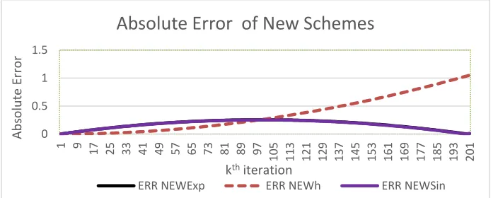
Fig 4: Graph of absolute Error for schemes in Fig. 3
0 0.1 0.2 0.3
1 9 17 25 33 41 49 57 65 73 81 89 97
105 113 121 129 137 145 153 161 169 177 185 193 201
Ab
so
lu
te
Erro
r
kthiteration
Absolute Error of New Schemes
ERR NEWExp ERR NEWh ERR NEWSin
0 5 10 15 20 25
1 9 17 25 33 41 49 57 65 73 81 89 97
105 113 121 129 137 145 153 161 169 177 185 193 201
y(t
k
)
kthiteration
Graph of New schemes with h=0.01
ANALYTIC NEWEXP NEWh NEWSINr
0 0.5 1 1.5
1 9 17 25 33 41 49 57 65 73 81 89 97
105 113 121 129 137 145 153 161 169 177 185 193 201
Ab
so
lu
te
Erro
r
kthiteration
Absolute Error of New Schemes
Fig 5: Graph of absolute Error for schemes in Fig. 3
5.0 DISCUSSION AND CONCLUSION
The derived simulation models have been tested with the control parameters ∝ and β. We also
applied the Non-Standard method by modifying denominator function which also provide have
parameters λ and r that can be chosen to obtain iteratively assigned step size as denominator. The
discrete model worked for only those models that assumed negligible air resistance, but it failed
for the other models of this dynamical phenomena. We therefore present the application of the
schemes to two initial value problems which are two different models of the evaporating
raindrop. The solution curves of the schemes follow the analytical solutions of the respective
equations monotonically as shown in Figs. 1and 3. The numerical properties of the schemes like
linear stability, convergence and consistency has been proved analytically. During the course of
simulating the equations we varied this control parameters to obtain family of curves that are
very close to the analytic solution and also have the same dynamics as the original equation. The
scheme NEWh is the Standard scheme because the denominator function remains the step size
throughout the iteration processes, but this scheme possesses the highest absolute error of
deviation from the analytic solution, this confirms the good qualities of Non-standard modeling.
The choice of appropriate values for variables λ and r can be determined using the conditions set
by Angueluv, Lubuma [5] and extended by Obayomi, Oke [9]. The graph of Absolute error (see
Figs 2, 4, 5) has demonstrated this quality. The same values of these parameters were used to
execute the iterations. The schemes of Model II produced absolute errors of less than 0.03. The
result of the schemes is consistent with literature. We can conclude that the discrete model can
be used to simulate the dynamics of evaporating raindrop as proposed.
0 0.1 0.2 0.3
1 10 19 28 37 46 55 64 73 82 91
100 109 118 127 136 145 154 163 172 181 190 199
Ab
so
lu
te
Erro
r
kthiteration
Absolute Error of New Schemes
CONFLICT OF INTERESTS
The authors declare that there is no conflict of interests.
REFERENCES
[1] Henrici P. Discrete Variable Methods in ODE. John Willey & Sons, New York. 1962.
[2] Fatunla S. O. Numerical Methods for Initial Values Problems on Ordinary Differential Equations. Academic Press, New York. 1988.
[3] Humphreys, W. J. Physics of the Air, 279, New York: Dover, 1964.
[4] Mickens R. E. Non-standard Finite Difference Models of Differential Equations. World Scientific, Singapore. 115, 144-162, 1994.
[5] Anguelov, R, and Lubuma J.M.S. Nonstandard finite difference method by nonlocal approximation. Math. Comput. Simul. 6(2003), 465-475.
[6] D.G. Zill and R.M. Cullen Differential Equations with boundary value problems (sixth Edition) Brooks /Cole Thompson Learning Academic Resource Center. 2005, pp. 90 -101.
[7] Riel, Herbert. Introduction to the Atmosphere. 3rd ed. New York: McGraw Hill, 1978: 107 [8] T. P. Dreyer. Modelling with Ordinary Differential Equations. CRC Press, New York, 1993.