T
HE
E
FFECT OF
P
OVERTY
S
TATUS AND
P
UBLIC
H
OUSING
R
ESIDENCY ON
R
ESIDENTIAL
E
NERGY
C
ONSUMPTION IN THE
U.S.
R
ASHA
A
HMED
Trinity College, United States
K
EELY
J
ONES
S
TATER
Public and Affordable Housing Research Corp, Unites States
M
ARK
S
TATER
Trinity College, United States
ABSTRACT
We use the U.S. Residential Energy Consumption Survey (RECS) for 2001 and 2005 to estimate household energy demand as a function of a composite energy price. We find a short-run price elasticity of -0.6 and a short-run income elasticity of 0.04 in the full sample, with poverty-level households having slightly higher price elasticities and lower income elasticities. Public housing residents use about 10% less energy than non-residents, a difference that persists despite a large set of household and dwelling controls and even with the analysis restricted to poverty-level households, multifamily housing occupants, and renters. Thus, the findings suggest that energy conservation measures undertaken by housing authorities have been effective at reducing energy consumption relative to similarly-situated households. Analysis by fuel type and use suggests that the relatively low energy use by public housing residents compared to other multifamily renters is driven by their lower use of natural gas for space heating, and electricity and natural gas for appliances.
JEL Codes: Q41, Q48, I32, R38
Keywords
Energy demand; Public housing; Low-income households
Corresponding Author:
Mark Stater, Trinity College, Dept of Economics, 300 Summit Street, Hartford CT USA
1. INTRODUCTION
Recent increases in energy prices and the lingering recession have made energy expenditures an important concern for many households across the United States. The poor especially have felt the burden of this increase as energy spending makes up a larger portion of their total household budget. Indeed, requests for energy assistance from low-income households have reached record numbers and are expected to rise (NEADA, 2009). How the energy needs of low-income households will respond to these current economic difficulties is an important policy question, yet we currently know relatively little about the determinants of energy consumption or the price and income responsiveness of energy demand among the poor and those receiving social assistance. This is the case despite the large volume of research on energy demand in general, some of which suggests energy use patterns differ by income (Colton, 2002).
We are particularly interested in the impact of housing subsidies on energy demand among low-income renter families and the possibility that living in subsidized housing can mediate low-income families’ energy consumption patterns. Low-income families in search of affordable housing can choose to live in 1) privately-owned properties that receive federal assistance to provide low-cost housing to qualifying individuals, 2) publicly-owned housing properties, 3) privately-owned properties whose landlords accept housing vouchers provided to qualifying residents, or 4) un-subsidized private housing. Of these four options, we focus on the impact on energy consumption of living in publicly-owned housing properties since on average, public housing properties are most closely monitored for quality and most frequently updated (HUD, 2005). And over the last decade, the Department of Housing and Urban Development (HUD), the Department of Energy (DOE), and public housing authority (PHA) managers have made substantial efforts to retrofit public housing properties and increase their energy efficiency (HUD, 2006; 2008). Whereas these actions should serve to reduce energy consumption for public housing residents, the implicit subsidy residents receive while living in public housing might lead to higher energy consumption, and thus it is an open empirical question what effect residency in public housing projects has on the consumption of energy.
Our empirical approach is to specify total energy demand at the household level across five component fuels as a function of a composite price of these fuels, household income, and other household and dwelling attributes. We then estimate the demand function using the 2001 and 2005 versions of the Residential Energy Consumption Survey (RECS) and obtain estimates of the price and income elasticities of energy demand for the full sample and various poverty-level subgroups to place the study into the context of the residential energy demand literature.
indicating that they place a high marginal value on energy use but may have priorities in their family budgets that are more pressing than additional energy use. Public housing residents use about 10% less energy than non-residents, ceteris paribus, a difference that holds up despite the inclusion of a lengthy set of household and dwelling controls and even when the analysis is restricted to poverty-level households, multifamily housing occupants, and renters – households we expect to be similar to public housing residents in attributes that affect energy use. Thus, the findings suggest that publicly-provided housing can mediate low-income energy use. The findings also offer indirect evidence that the energy conservation and efficiency measures undertaken by HUD and local housing authorities have been effective at reducing energy consumption among residents relative to other households in similar income and housing circumstances. Analysis that is disaggregated by fuel type and use suggests that the lower energy use by public housing residents relative to other multifamily renters is driven primarily by lower use of natural gas for space heating, and of electricity and natural gas for appliances. These findings support structural improvements to public housing buildings, upgrades to the efficiency of the appliance stock, and discretionary choices of residents as reasons for relatively low energy use.
2. RELATED LITERATURE
The literature on residential energy demand is sufficiently vast that it has been surveyed or meta-analyzed numerous times (Taylor 1975; Berndt 1978; Bohi 1981; Bohi and Zimmerman 1984; Dahl 1993; Espey and Espey 2004; Kristrom 2008; van den Bergh 2008; Swan and Ugursal 2009). As these surveys discuss, a central problem in energy demand analysis is that due to the non-constant block rate pricing structure used by many electric utilities, price and quantity consumed are simultaneously determined for the consumer, which means the price variable is endogenous in the demand equation. This pricing structure also causes average and marginal price to differ, which leads to measurement error because economic theory suggests that the marginal price affects behavior, but most data sets only include information on the average price. Thus, many studies use instrumental variables to correct for the endogeneity of price, although some use data from experiments in which price changes are unrelated to consumer behavior.
A problem with data that is aggregated beyond the household level is that it may fail to capture the microeconomic determinants of electricity demand. Thus, many studies use micro data to examine the influence of prices, incomes, and other household and dwelling attributes on electricity demand (Wilder and Willenborg, 1975; Parti and Parti, 1980; Barnes, Gillingham and Hagemann, 1981; Archibald, Finifter, and Moody, 1982; Garbacz, 1983; Henson, 1984; Dubin and McFadden, 1984; Branch, 1993). The bulk of the short-run price elasticity estimates from these micro-econometric studies are from -0.2 to -0.7, and the long-run price elasticities are from -0.25 to -1.4. The short-run and long-run income elasticities are from 0.03 to 0.28 and from 0.02 to 0.4, respectively.
Hirst, Goeltz, and Carney (1982) take an approach similar to ours, using the National Interim Energy Consumption Survey, a forerunner of the RECS, to estimate total energy use as a function of the average prices of component fuels. They find a price elasticity that ranges between -0.4 and -0.7 and an income elasticity of about 0.08. O’Neill and Chen (2002) find based on RECS data from 1993 and 1994 that per-capita residential energy use increases with the age of the householder and the number of adults in the household and decreases in household size. Colton (2002) finds that families with low income use less energy than middle- or upper-income families, while Haas (1997) finds that lifestyle and demographic factors including income are among the key determinants of energy use. However, Brandon and Lewis (1999) find that income and other socio-demographics do not affect the changes in energy consumption arising from households receiving feedback on their consumption patterns (a phenomenon that tends to result in lower consumption in general).
Research has also considered how the price and income responsiveness of energy demand vary with the quantity of use (Wills, 1981; Faruqui and Malko, 1983; Reiss and White, 2005; Fan and Hyndman, 2011) and with household characteristics such as income (Baker, Blundell, and Micklewright, 1989; Nesbakken, 1999; Wilder, Johnson, and Rhyne, 1992; Fell, Li, and Paul, 2010), race (Poyer and Williams, 1993), age (Baker, Blundell, and Mickelwright, 1989), and owner/renter status (Baker and Blundell, 1991; Rehdanz, 2007). Reiss and White (2005) use the 1993 and 1997 versions of the RECS matched with data on actual utility rate structures to examine electricity demand in California. They find that the price elasticity is lower at higher quartiles of household income and electricity use. Poyer and Williams (1993) use RECS data for 1980, 1982, and 1987 to estimate electricity and total energy demand by race. They find that blacks are more price sensitive than whites in their electricity demand but less price sensitive in their total energy demand in both the short run and long run.
income brackets. Reiss and White (2005) find in their analysis of the RECS that, in California, households living in public housing consume less electricity than those in private housing. However, they do not examine whether this is true for the nation as a whole, for other fuels, or for total energy use. Rehdanz and Stowhase (2008) find that, in the German welfare system, having utilities paid for by the government increases electricity use for recipients by more than 5 percent.
Our approach extends the prior research on income and housing issues in the energy market by examining the effects of poverty status and public housing residency on total energy use and how the price and income responses of poverty-level households compare to the rest of the population. We estimate overall energy demand across all fuel types, the demand for each of the component fuels, and the demand for energy in various possible end uses for all households, those near the poverty line, multifamily occupants and renters.
3. DATA, EMPIRICAL METHODS, AND DESCRIPTIVE STATISTICS
3.1 Data
The data for this study come from the 2001 and 2005 versions of the Residential Energy Consumption Survey (RECS, 2001; 2005), which is collected by the Energy Information Administration (EIA) of the U.S. Department of Energy. The survey’s design is a multi-stage area probability sample that collects information on housing unit characteristics and energy consumption behaviors from a randomly selected group of households. Household demographic information is collected by interview, dwelling characteristics are obtained through observations made by the interviewers, and energy consumption and expenditure data are obtained directly from the power companies that supply these households. Our sample consists of 9040 households, of which 2496 have incomes below 150% of the federal poverty line, 1428 have incomes below 100% of the poverty line, and 358 reside in public housing projects.1
3.2 Empirical Methods
Our regression models for total energy consumption at the household level can be expressed in error form with the following equation:
Log Ei = αLog Pi + xiβ + ui, (1)
where Ei is total household energy consumption, Pi is the composite price of
energy faced by the household i, xi is a vector of household and dwelling
characteristics, and ui is a stochastic error term with mean zero. We estimate equation (1) for the full sample of individuals in the RECS survey, for the Poor 150 (households with incomes below 150% of the federal poverty line), the Poor 125 (incomes below 125% of the poverty line), the Poor 100 (incomes below 100% of the poverty line), households who live in multifamily buildings, and renters. The equations are estimated with OLS using standard errors that are robust to heteroskedasticity.
1 For reference, in 2005 the federal poverty line for the 48 contiguous states and the District of
The dependent variable Log Ei in our regressions is the natural log of the sum of
the household’s total combined consumption of electricity, natural gas, fuel oil, liquid propane, and kerosene in thousands of British Thermal Units (BTUs).2 Whereas the usual approach in most of the literature is to estimate the demand for a specific type of energy as a function of its price, the availability of information on multiple types of fuels in the RECS affords us the opportunity to gain a more comprehensive picture of household energy consumption by studying how total energy demand responds to the overall price of energy. This approach is relevant to policy discussions because the increasing strain on the world’s energy resources refers to multiple types of energy use, not just a single type, and the concern over the dependence of the U.S. on foreign energy sources is in part a concern about the total amount of energy we consume. Furthermore, since households are able to substitute between different types of energy, knowing that just one type of energy use is decreasing in response to a price change does not assure us that energy use as a whole is changing. Thus, in order to develop a broader understanding of how households respond to overall trends in energy prices it is useful to consider total energy demand.3 However, we also estimate versions of equation (1) for each specific fuel and several different end-uses of energy to be consistent with the literature.4 We also break end uses down by specific fuel types.
The explanatory variables in the vector xi include income, measures of
socioeconomic status and public assistance (dummy variables for utilities included in the rent; receipt of cash benefits; receipt of noncash benefits; LIHEAP assistance; rental assistance; renting one’s home; living in public housing), demographic controls (respondent’s age, sex, and race; size of household), geographic controls (region of the U.S.; heating degree days; cooling degree days), characteristics of the dwelling (square feet; building age; number of rooms; dummy for multifamily housing; dummy for poor insulation) and household appliances (number of major appliances; dummy for swimming pool; number of personal computers; number of color televisions; dummy for central air conditioning; dummy for window- or wall-mounted air conditioning; average age of major appliances), and survey year (dummy for 2001). A list of these variables and a brief description of each one is provided in Table 1. Note that the income data recorded in the RECS are categorical, so to obtain a continuous measure of income we simply assign each household the midpoint of the income category it occupies in its respective survey year. Detailed information on the income categories can be found in Table 1.
2 A demand specification of the form (1) can be rationalized in theory based on a Cobb-Douglas
household utility function across the different types of energy. But, the construction of the composite price suggested by Cobb-Douglas utility is slightly different than the one we actually use for reasons explained below (footnote 6).
3 Our results are largely driven by consumption of electricity and natural gas. Virtually everyone in
the sample uses electricity, and over 60% use natural gas. Only about 11% use propane, 10% use fuel oil, and 2% use kerosene. In addition, most of the substitution possibilities actually practiced by households appear to be along the lines of electricity vs. natural gas, or each non-electric fuel vs. electricity. Few households that use electricity also use anything other than natural gas, and few households that use a non-electric fuel also use a second non-electric fuel.
4 It is also the case that, since we lack data on the set of fuels each household is hooked up to use,
Table 1: Descriptions of Variables
Variable Description
Energy Consumption Total annual household electricity, natural gas, fuel oil, liquefied petroleum gas, and kerosene use in thousands of British Thermal Units
Energy Price Consumption-weighted average of the prices (per 1000 BTU) of electricity, natural gas, fuel oil, liquefied petroleum gas, and kerosene faced by household
Household Income
Annual household income in dollars; value assigned is midpoint of the household’s income category, where the categories for the 2001 survey are 0-4999, 5000-9999, 10000-14999, 15000-19999, 20000-29999, 30000-39999, 40000-49999, 50000-74999, 75000-99999, and 100000+. Households in the 100000+ category are assigned an income of 100000. The categories for the 2005 survey are: 0-2499, 2500-4999, 5000-7499, 7500-9999, 10000-14999, 15000-19999, 20000-24999, 25000-29999, 30000-34999, 35000-39999, 40000-44999, 45000-49999, 50000-54999, 55000-59999, 60000-64999, 65000-69999, 70000-74999, 75000-79999, 80000-84999, 85000-89999, 90000-94999, 95000-99999, 100000-119999, and 120000+. Households in the 120000+ category are assigned an income of 120000.
Utilities in Rent Dummy variable = 1 if some or all utility costs are included in household’s rent
Cash Benefits Dummy variable = 1 if household receives cash benefits from Temporary Assistance for Needy Families, Supplemental Security Income, general assistance, or other public assistance Non-cash Benefits Dummy variable = 1 if household receives non-cash benefits from food stamps or public/subsidized housing
Liheap Assistance
Dummy variable = 1 if household receives assistance under the Low Income Home Energy Assistance Program. Eligibility is determined by each state based on household income and household size.
Rental Assistance Dummy variable = 1 if household receives rental assistance Renter Dummy variable = 1 if household rents the dwelling where it resides Public Housing Dummy variable = 1 for public housing residents
Age Householder Age of the householder in years
HH Size Number of individuals in the household Square Feet Total size of dwelling in square feet
Total # of Rooms Total number of rooms in the dwelling (bedrooms, bathrooms, other rooms) Building Age Age of building (back to 1940)
Multi-Family Dummy variable = 1 if building household occupies contains 2 or more apartments
Swimming Pool Dummy variable = 1 if residence has a swimming pool for household’s private use
Poor Insulation Dummy variable = 1 if residence is poorly insulated or has no insulation
Number of PCs Number of personal computers in the dwelling Num. of Color TVs Number of color TVs in the dwelling
Central A/C Dummy variable = 1 if dwelling has central air conditioning Window or Wall A/C Dummy variable = 1 if dwelling has window- or wall-mounted air conditioning units Female Dummy variable = 1 if householder is female
Northeast Dummy variable = 1 if household lives in the northeast census region (the states of CT, ME, MA, NH, VT, RI, NJ, NY, and PA)
Midwest Dummy variable = 1 if household lives in the midwest census region (the states of IL, IN, MN, OH, WI, IA, KS, MO, NE, ND, and SD)
West Dummy variable = 1 if household lives in the west census region (the states of AZ, CO, ID, MT, NV, NM, UT, WY, AK, CA, HI, OR, and WA)
South Dummy variable = 1 if household lives in the south census region (Washington, D.C. and the states of DE, FL, GA, MD, NC, SC, VA, WV, AL, KY, MS, TN, AR, LA, OK, and TX)
Heating Degree Days Total number of degrees per annum that the mean daily temperature in the household’s location of residence falls below 65 degrees Fahrenheit
Cooling Degree Days Total number of degrees per annum that the mean daily temperature in the household’s location of residence rises above 65 degrees Fahrenheit
Avg. Age Appliances Average age of the major appliances in the residence White Dummy variable = 1 if householder self-identifies as white Asian Dummy variable = 1 if householder self-identifies as Asian Black Dummy variable = 1 if householder self-identifies as black Hispanic Dummy variable = 1 if householder self-identifies as Hispanic
Other Dummy variable = 1 if householder self-identifies as a member of some other race (e.g., Native American, Hawaiian or Pacific Islander)
Year 2001 Dummy variable = 1 if household is interviewed in the 2001 version of the RECS
Year 2005 Dummy variable = 1 if household is interviewed in the 2005 version of the RECS
The energy price variable Pi is a composite measure of the average prices faced by
the household for electricity, natural gas, fuel oil, liquid propane, and kerosene. The variable is constructed as a consumption-weighted average of the prices of the fuels that the household actually consumes (since the prices of fuels it does not consume are unavailable in the data), where the weights are the ratios of consumption of each type of fuel to total energy consumption in the full sample for the respective survey year (2001 or 2005).5,6 The precise definition of the composite price variable for household i is therefore given by:
Pi = ΣjWjpji / ΣjWjIji, (2)
where Wj is the weight for fuel type j (j = electricity (EL), natural gas (NG), fuel oil (FO), liquid propane (LP), or kerosene (KER)), pji is the average price of fuel j
facing household i and Iji is an indicator variable that equals 1 if household i
consumes a positive amount of fuel j and equals 0 otherwise. The price pji that the
household faces for fuel type j (per 1000 BTUs) is not directly reported in the data, but is constructed by dividing the total dollar amount spent on type j during the year by the total amount of type j consumed (in 1000s of BTUs). If the household does not consume any of type j we set pji equal to zero so as to exclude this price from
the weighted average calculation (and then because of the indicator functions in the denominator the weight for this type of fuel is also excluded from the denominator of the expression). Taking the ratio of consumption of each type of fuel to total energy consumption in the sample for each survey year, we obtain the following weights for 2001: WEL = 0.3804, WNG = 0.4723, WFO = 0.0971, WLP = 0.0445, and
WKER = 0.0056. For 2005, the weights are WEL = 0.3946, WNG = 0.4523, WFO =
0.1039, WLP = 0.0476, and WKER = 0.0016.
The use of the average price to explain demand raises two potential problems. First, economic theory suggests that the consumer responds to the marginal price, which differs from the average price under the declining or increasing block schedules used by many power suppliers. Furthermore, under non-constant block pricing, differences in marginal prices between adjacent consumption blocks affect the consumer’s net income, so theoretically the change in income due to the movement away from the previous block (called an “inframarginal demand charge” or a “rate structure premium”) should also be included in the demand equation.
A number of studies, however, have provided rationales for simply using the average price. Halvorsen (1975) shows that, assuming log-linear functional forms, the elasticities obtained from using the average price are identical to those obtained with the marginal price. Shin (1985) argues that consumers may actually respond to average rather than marginal prices due to information costs. Smith (1980) argues based on RESET results for a national sample that statistically valid estimates need not require information on marginal and inframarginal prices, but can be obtained using (instrumented) average revenue prices. Borenstein (2009) finds that the observed consumption distribution among consumers in southern California is not consistent with them having an accurate understanding of the marginal prices that they face under an increasing-block schedule. This is because unexpected demand shocks make it difficult for them to know what the relevant marginal price will be. Instead they appear to respond to expected marginal prices, though the average price is also a reasonably good predictor.
6 We experimented with various ways of constructing the weights. When we use the household’s own
The second problem is that, even if the average price is the correct price to use, it is potentially endogenous because it depends on quantity consumed under non-constant block pricing.7 However, this may be mitigated somewhat by our approach of constructing a composite price across multiple types of fuels sold under different tariff structures, and using fuel weights based on consumption patterns in the full sample rather than just for the household.8 Indeed, when we formally test our composite average price variable for endogeneity, the null hypothesis of exogeneity is not rejected in virtually every case. Nonetheless, to address the possibility that an undetected endogeneity problem still remains, we also instrument for the price of energy faced by the household using the population-weighted average energy price among states within the household’s census division. Note that the RECS data do not report the exact state in which the household resides unless it is in one of the four largest states of New York, California, Texas, or Florida. For these states we simply take the average energy price within the state. Thus, for each state we compute a composite average energy price by taking a consumption-weighted average of the state average prices of each of the component fuels. These state-level component fuel prices are available from the State Energy Data System (SEDS) collected by the United States Energy Information Administration (U.S. EIA, 2010). We compute the instruments separately for each of our survey years using the 2000 and 2004 versions of the SEDS series.
To be precise about how the instruments are constructed, let psj denote the
average price of fuel j in state s (for a specific year). Let Csj denote the total consumption of fuel j in state s for that same year, so that Cs ΣjCsj is the total
consumption of all fuels in state s. Then wsj Csj/Cs is the share of total energy
consumption in state s devoted to fuel j. The composite energy price in state s is then the consumption-weighted average of the prices of the individual fuels in state
s: ps Σjwsjpsj. Now let Nsk denote the population of state s in census division k and let Nk ΣsNsk be the total population of division k, so that πsk Nsk/Nk is the share of division k’s population living in state s. Then the composite price of energy for division k, which is used as the instrument for the household-level composite price for all households in that division, is the population-weighted average of the composite energy prices for the states in the division: pk Σsπskps.
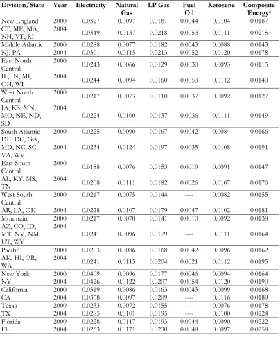
For reference, the names of the census divisions, the states within each of the divisions, and the average price of each type of fuel for each division are presented in Table 2. Note that the divisional average price of fuel type j in these tables is
7 Historically electric utilities primarily used decreasing block pricing, but recently some have moved
toward the opposite approach of increasing block pricing (Borenstein, 2009). Having a sample in which some consumers face either of these two pricing schemes may help reduce the endogeneity problem in energy demand estimation, since the decreasing and increasing block structures may effectively cancel each other out so that quantity consumed is approximately uncorrelated with price in the population.
8 Note that because only the prices of the fuels that the household actually consumes are averaged
constructed as the population-weighted average of the price of fuel j for states within the division: pjk Σsπskpsj. These are used to construct the divisional
composite prices listed in the table by taking consumption-weighted averages across the divisional average prices of the individual fuels: qk Σjλjkpjk, where λjk is the
share of total energy consumption across all fuels in division k devoted to fuel j. These divisional composite prices are not identical to the instruments pk described above and used in the analysis, but they are more convenient to present in tabular form and also lead to similar instrumental variables (IV) results as the pk. In
addition, the prices pjk that form the qk are used to develop instruments for the division-specific composite energy prices utilized in the section below on energy consumption by type of end use.
Table 2: Fuel Prices by Census Divisiona,b
Division/State Year Electricity Natural
Gas LP Gas Fuel Oil Kerosene Composite Energyc
New England 2000 0.0327 0.0097 0.0181 0.0044 0.0104 0.0187
CT, ME, MA,
NH, VT, RI 2004 0.0349 0.0137 0.0218 0.0053 0.0111 0.0215
Middle Atlantic 2000 0.0288 0.0077 0.0182 0.0043 0.0088 0.0143
NJ, PA 2004 0.0301 0.0115 0.0213 0.0052 0.0120 0.0178
East North
Central 2000 0.0243 0.0066 0.0129 0.0030 0.0093 0.0115
IL, IN, MI,
OH, WI 2004 0.0244 0.0094 0.0160 0.0053 0.0112 0.0140
West North
Central 2000 0.0217 0.0073 0.0110 0.0037 0.0092 0.0127
IA, KS, MN, MO, NE, ND, SD
2004
0.0224 0.0100 0.0137 0.0036 0.0111 0.0149
South Atlantic 2000 0.0225 0.0090 0.0167 0.0042 0.0084 0.0166
DE, DC, GA, MD, NC, SC,
VA, WV 2004 0.0234 0.0124 0.0197 0.0035 0.0108 0.0191
East South
Central 2000 0.0188 0.0076 0.0153 0.0019 0.0091 0.0147
AL, KY, MS,
TN 2004 0.0208 0.0111 0.0182 0.0026 0.0107 0.0176
West South
Central 2000 0.0217 0.0075 0.0144 ---- 0.0082 0.0155
AR, LA, OK 2004 0.0228 0.0107 0.0179 0.0047 0.0102 0.0181
Mountain 2000 0.0217 0.0070 0.0141 0.0010 0.0092 0.0138
AZ, CO, ID, MT, NV, NM, UT, WY
2004
0.0241 0.0096 0.0179 ---- 0.0111 0.0164
Pacific 2000 0.0203 0.0086 0.0168 0.0042 0.0096 0.0162
AK, HI, OR,
WA 2004 0.0241 0.0115 0.0204 0.0021 0.0112 0.0195
New York 2000 0.0409 0.0096 0.0177 0.0046 0.0094 0.0164
NY 2004 0.0426 0.0122 0.0207 0.0054 0.0120 0.0190
California 2000 0.0319 0.0086 0.0163 0.0043 0.0099 0.0168
CA 2004 0.0358 0.0097 0.0209 ---- 0.0116 0.0189
Texas 2000 0.0233 0.0072 0.0155 ---- 0.0076 0.0178
TX 2004 0.0285 0.0101 0.0195 ---- 0.0100 0.0224
Florida 2000 0.0228 0.0117 0.0193 0.0044 0.0090 0.0222
Notes: aAll prices are in dollars per thousand BTUs. bThe price of a particular fuel for a division is
calculated as the population-weighted average of the average prices of that fuel for the states within the division. State-level price data are from the U.S. Energy Information Administration (2010) and state-level population data are from the U.S. Census Bureau (2012a). cComposite energy price for a division
is constructed as a consumption-weighted average of the prices of the individual fuels for the division. State-level consumption data are obtained from the Energy Information Administration (2010).
Despite the fact that by construction there is absolutely no variation in the instruments for households in the same census division, these instruments perform relatively well. They generally produce statistically significant estimates of price elasticities and are reasonably predictive of the household-level price variable. Indeed, in most of the specifications we estimate the R-squared values for the first stage regressions are well above one-third. Since the IV results for the price elasticities tend to be larger than the corresponding OLS estimates, OLS is used as our preferred approach throughout most of the analysis. It yields more conservative results on price responses, similar results to IV for other variables, and uses a household price variable that is found to be exogenous to energy use in virtually every formal test that we conduct.
3.3 Descriptive Statistics
Descriptive statistics for the variables utilized in our analysis are presented in Table 3 below. We present separate means for the entire sample, the Poor 100, multifamily renters, and those in public housing. We also test for significant differences in means between those who are and are not in each of these groups, as indicated by the stars in the table. The results for the full sample indicate that the average total energy consumption in the sample is 96,445 thousand BTUs (kilo-BTUs or k(kilo-BTUs) and that the average composite energy price is about $0.023 per kBTU. This implies an average total energy bill of $2,210 per year, or $184 per month. The Poor 100, multifamily residents and those who live in public housing consume far less energy than households outside these groups. For multifamily renters and public housing residents, the average values of energy consumption are only 57,708 and 55,683 kBTUs, respectively. The means also indicate that the Poor 100, multifamily renters, and those in public housing are much more likely than people not in these groups to receive various forms of social assistance, to have utilities costs included as part of their rent, and to be headed by female householders. They are much less likely to have central air conditioning systems and swimming pools, and more likely to have window- or wall-mounted air conditioning units. People in these groups are also more likely to be nonwhite; they have lower incomes, live in much smaller dwellings with fewer rooms, own fewer and older major appliances, and own fewer personal computers and color TVs than people who are not in these groups. Multi-family renters and public housing residents live in slightly newer buildings, whereas the poor 100 live in older buildings than households not in these groups.9 Public housing residents are no more or less likely to have poor insulation than non-residents, but the poor 100 and multi-family
9 This is probably because our building age variable only dates back to 1940. Many single- and
renters in general are more likely to have poor insulation than people not in these groups.
Table 3: Descriptive Statistics
ALL POOR 100 MULTIFAMILY RENTERS HOUSING PUBLIC
Mean [SD] Mean [SD] Mean [SD] Mean [SD]
Energy Consumpti
on 96,445 [56,642] 79,076** [52,069] 57,708** [42,255] 55,683** [36,654]
Energy
Price 0.023 [0.008] 0.023 [0.011] 0.025** [0.009] 0.022 [0.007]
Household
Income 45,390 [31,492] 9,589** [5,216] 29,299** [24,327] 14,857** [12,237]
Utilities in
Rent 0.044 [0.204] 0.107** [0.309] 0.175** [0.380] 0.302** [0.460]
Cash
Benefits 0.069 [0.254] 0.260** [0.439] 0.140** [0.347] 0.324** [0.469]
Non-cash
Benefits 0.084 [0.277] 0.369** [0.483] 0.204** [0.403] 0.508** [0.501]
Liheap
Assistance 0.354 [0.478] 1.0** [0.0] 0.566** [0.496] 0.858** [0.350]
Rental
Assistance 0.028 [0.164] 0.113** [0.316] 0.093** [0.291] 0.0** [0.0]
Renter 0.314 [0.464] 0.612** [0.487] 1.0** [0.0] 1.0** [0.0]
Public
Housing 0.040 [0.195] 0.148** [0.356] 0.159** [0.366] 1.0** [0.0]
Age HH
Head 49.3 [17.3] 49.6 [19.8] 43.3** [18.9] 50.3 [21.0]
HH Size 2.65 [1.48] 2.76** [1.80] 2.24** [1.35] 2.15** [1.49]
Square Feet 2,188 [1,510] 1,380** [1,033] 923** [501] 896** [534]
Total # of
Rooms 6.56 [2.33] 5.22** [1.83] 4.36** [1.43] 4.25** [1.44]
Building
Age 36.4 [20.2] 40.4** [19.8] 37.6** [19.5] 34.5~ [17.2]
Multi-Family 0.228 [0.419] 0.408** [0.492] 1.0** [0.0] 0.782** [0.413]
Swimming
Pool 0.065 [0.247] 0.011** [0.105] 0.0** [0.0] 0.0** [0.0]
Poor
Insulation 0.198 [0.398] 0.315** [0.465] 0.235** [0.424] 0.207 [0.406]
# of Major
Appliances 4.94 [1.47] 3.86** [1.32] 3.36** [1.23] 3.13** [1.10]
Number of
PCs 0.89 [0.95] 0.42** [0.71] 0.60** [0.83] 0.30** [0.558]
Number of
Color TVs 2.38 [1.25] 2.02** [1.12] 1.77** [0.94] 1.80** [0.93]
Central
A/C 0.517 [0.500] 0.312** [0.464] 0.359** [0.480] 0.358** [0.480]
Window or
Wall A/C 0.257 [0.437] 0.371** [0.483] 0.366** [0.482] 0.344** [0.476]
Female 0.567 [0.496] 0.688** [0.463] 0.593* [0.491] 0.690** [0.463]
Northeast 0.222 [0.416] 0.210 [0.408] 0.290** [0.454] 0.268* [0.444]
West 0.244 [0.429] 0.242 [0.429] 0.271** [0.445] 0.196* [0.397]
South 0.316 [0.465] 0.350** [0.477] 0.252** [0.434] 0.318 [0.467]
Heating Degree
Days 4,269 [2,104] 4,098** [2,032] 4,189
~ [2,031] 4,188 [1,849]
Cooling Degree
Days 1,405 [979] 1,476** [932] 1,348** [979] 1,337 [823]
Avg. Age
Appliances 9.53 [5.14] 10.23** [6.11] 9.87** [6.01] 10.15* [7.01]
Asian 0.030 [0.169] 0.024 [0.153] 0.054** [0.226] 0.045~ [0.207]
Black 0.117 [0.321] 0.231** [0.422] 0.187** [0.390] 0.282** [0.451]
Hispanic 0.059 [0.236] 0.119** [0.324] 0.112** [0.316] 0.073 [0.260]
Other Race 0.045 [0.207] 0.073** [0.260] 0.069** [0.253] 0.087** [0.282]
White 0.750 [0.433] 0.553** [0.497] 0.578** [0.494] 0.514** [0.501]
Year 2001 0.515 [0.500] 0.458** [0.498] 0.532 [0.499] 0.472~ [0.500]
Year 2005 0.485 [0.500] 0.542** [0.498] 0.468 [0.499] 0.528~ [0.500]
N 9040 1428 1761 358
**Significantly different from the mean for those not in the category (poor 100, multi-family renters, or public housing, respectively) at the .01 level, *at the .05 level, ~at the .10 level. Descriptions of all variables provided
in Table 1.
4. RESULTS
4.1 Energy Consumption for the Full Sample and Poor Households
In Table 4 we present the OLS estimates of the energy consumption model (1) for the full sample, for the Poor 150, the Poor 125, and the Poor 100. The results for the full sample indicate that the price elasticity of energy demand is -0.59 according to OLS and -0.70 according to IV. Both values are well within the interval spanned by the bulk of the micro-econometric estimates. The estimated income elasticity is 0.036, which is smaller than most but not all of the short-run estimates in the literature, perhaps reflecting measurement error resulting from the assignment of the midpoint income value to everyone in the same category. Thus, this is probably best interpreted as a lower-bound estimate of the short-run income elasticity of energy demand.
The results for the full sample also indicate that the receipt of non-cash benefits increases energy consumption by 7.4 percent, but that energy consumption does not respond to cash benefits, LIHEAP assistance, rental assistance, or having the costs of utilities included in the rent. The latter result may reflect that when utilities are included in the rent households often are not allowed to control the thermostat. Renters in general do not consume significantly different amounts of energy than owners, but households living in public housing consume 10.5 percent less energy than those not in public housing, all other factors held constant. Considering the relatively large number of control variables in our regression, this suggests that living in public housing has the effect of reducing a household’s energy use.10 Since rental assistance in general has no effect on energy consumption, it appears that the
10 It is possible to also control for the material that the structure is made out of (brick, wood, siding,
type of public subsidy a household receives is critical for determining its total energy use. This may be because HUD and PHAs have over the last decade undertaken a variety of energy-efficiency initiatives such as the retrofit and modernization of old properties, the purchase of energy star appliances, the weatherization of units, the provision of incentives for energy-efficient construction, and the incorporation of energy conservation measures into public housing utility funding formulas (Abt Associates, 1998; HUD, 2006). However, there may also be differences in unobserved attributes that affect energy use between those who do and do not reside in public housing, such as “thriftiness” in the purchases of basic goods, a possibility we further explore when we analyze the various poverty-level groups, multifamily housing occupants, and renters, who are likely to be much more similar to public housing residents on unobserved characteristics than is the population in general.
Table 4: OLS Analysis of Total Household Energy Consumption by Income Dependent Variable = log of total annual energy consumption (electricity, natural gas, propane, fuel oil, kerosene)
ALL POOR 150 POOR 125 POOR 100
Variables Coeff. [SE] Coeff. [SE] Coeff. [SE] Coeff. [SE]
Log Energy
Price -0.593** [0.027] -0.628** [0.050] -0.646** [0.064] -0.646** [0.074]
Log Price
(IV Est.)a -0.699** [0.082] -0.758** [0.171] -1.041** [0.228] -1.097** [0.284]
Log Incomeb 0.036** [0.011] 0.013 [0.018] 0.018 [0.021] 0.009 [0.025]
Utilities in
Rent 0.013 [0.029] 0.038 [0.039] 0.012 [0.047] 0.020 [0.052]
Cash
Benefits -0.002 [0.025] -0.010 [0.031] -0.017 [0.035] -0.012 [0.038]
Non-cash
Benefits 0.074** [0.026] 0.056~ [0.031] 0.057 [0.035] 0.058 [0.039]
Liheap
Assistance 0.012 [0.017] ---- ---- ---- ---- ---- ----
Rental
Assistance -0.011 [0.038] -0.020 [0.046] -0.035 [0.053] -0.029 [0.058]
Renter 0.007 [0.016] -0.022 [0.029] -0.004 [0.036] -0.010 [0.044]
Public
Housing -0.105** [0.031] -0.129** [0.037] -0.140** [0.041] -0.121** [0.046]
Age of
Householder 0.006** [0.002] 0.007* [0.003] 0.007 [0.004] 0.006 [0.004]
Age2/1000 -0.042* [0.017] -0.060* [0.030] -0.058 [0.036] -0.051 [0.038]
HH Size 0.130** [0.012] 0.165** [0.022] 0.149** [0.025] 0.155** [0.029]
(HH
Size)2/10 -0.088** [0.015] -0.121** [0.024] -0.108** [0.027] -0.122** [0.032]
Log Square
Feet 0.105** [0.012] 0.105** [0.029] 0.076* [0.033] 0.093* [0.039]
Total #
Rooms 0.051** [0.004] 0.044** [0.010] 0.053** [0.012] 0.055** [0.014]
Building
Age/10 0.048** [0.003] 0.051** [0.006] 0.050** [0.007] 0.059** [0.008]
Multi-Family -0.185** [0.018] -0.190** [0.031] -0.178** [0.036] -0.170** [0.040]
Swimming
Poor
Insulation 0.040** [0.013] 0.067** [0.025] 0.063* [0.029] 0.062~ [0.033]
# Major
Appliances 0.071** [0.005] 0.070** [0.011] 0.058** [0.014] 0.060** [0.016]
Number of
Computers 0.018** [0.005] 0.013 [0.015] 0.010 [0.017] 0.020 [0.022]
Num. of
Color TVs 0.017** [0.004] 0.026* [0.010] 0.041** [0.013] 0.039** [0.015]
Central A/C 0.016 [0.016] 0.034 [0.032] 0.048 [0.038] 0.067 [0.044]
Window or
Wall A/C 0.037* [0.017] 0.048 [0.032] 0.055 [0.038] 0.072~ [0.043]
Householder
Female 0.008 [0.009] 0.044* [0.022] 0.043~ [0.026] 0.039 [0.031]
Northeast
Region 0.345** [0.021] 0.394** [0.044] 0.386** [0.054] 0.377** [0.062]
Midwest
Region 0.084** [0.016] 0.121** [0.035] 0.107* [0.044] 0.073 [0.050]
West Region -0.083** [0.015] -0.119** [0.033] -0.142** [0.041] -0.153** [0.048]
Heat. Deg.
Days/1000 0.065** [0.004] 0.078** [0.009] 0.083** [0.011] 0.084** [0.012]
Cool. Deg.
Days/1000 0.057** [0.007] 0.091** [0.017] 0.095** [0.020] 0.086** [0.023]
Avg. Age
Appliances -0.001 [0.001] 0.003 [0.002] 0.005* [0.002] 0.006* [0.003]
Householder
Asian -0.104** [0.029] -0.065 [0.070] -0.026 [0.087] -0.035 [0.107]
Householder
Black 0.163** [0.016] 0.191** [0.029] 0.182** [0.034] 0.182** [0.039]
Householder
Hispanic 0.017 [0.023] 0.046 [0.036] 0.069 [0.044] 0.092~ [0.052]
Householder
Other -0.004 [0.025] 0.043 [0.038] -0.016 [0.046] -0.037 [0.053]
Year 2001 -0.210** [0.013] -0.190** [0.028] -0.210** [0.036] -0.219** [0.041]
Constant 6.179** [0.172] 6.029** [0.313] 6.073** [0.359] 6.024** [0.410]
N 9040 2496 1794 1428
R-squared 0.604 0.573 0.565 0.560
** Statistically significant at the .01 level, *at the .05 level, ~at the .10 level. Standard errors robust to
heteroskedasticity.
Notes: aInstrument for energy price is the population-weighted average energy price among states within the
census division. The average energy price within each state is computed as a consumption-weighted average of the state average prices of electricity, natural gas, propane, fuel oil, and kerosene as obtained from the U.S. Energy Information Administration (2010). bIncome variable created by assigning each household the midpoint
income value in its income category. The income categories are listed in Table 1.
insulated. The presence of window- or wall-mounted air conditioning units increases energy use, but the presence of central air conditioning does not. This may be because central air conditioning is thermostat-controlled and ceases to operate once the targeted temperature is achieved. Finally, energy consumption in 2001 is estimated to be 21 percent lower than in 2005, all else equal. Whereas the raw difference in energy use between the two years is only about 3 percent (95,030 kBTUs vs. 97,950 kBTUs), the controlled difference is much larger, perhaps because of increases in energy prices and decreases in the number of rooms per residence, the mean age of buildings, and the number of major appliances per residence that took place between 2001 and 2005.
Looking separately at the OLS results for the poverty groups, we see that all of them have price responses that are similar to but slightly larger in magnitude than those of the full sample. According to the IV results the responses are much larger for the poverty groups, especially the Poor 125 and Poor 100; in fact they are approximately unit elastic for these groups. For the income response the situation is the exact opposite: the poverty groups are all less responsive to income than the sample as a whole; in fact the income elasticity is not significantly different from zero for any of the poverty groups. These results suggest that poor households place a high marginal value on energy consumption with income held constant, but do not wish to devote increases in their income to additional energy use. It may be that, while energy serves a useful function for poor households (e.g. it allows them to more easily engage in activities that they desire), other items in the household budget (such as food and housing) have greater priority and are allocated the bulk of any increases in income that these families experience. Only when there is a decrease in relative prices do these households substitute toward more energy use.
Among the Poor 150, those in public housing consume 12.9 percent less energy than those in private housing, which suggests that the negative effect of living in public housing is not likely due to public housing residents being concentrated at lower values of income within each of our income categories or having lower unobserved wealth than those in private housing. But, it is still possible that there are differences in unobserved characteristics related to energy use between residents and non-residents, even among the very poor. Nevertheless, when we estimate the model for the Poor 125 and the Poor 100 for whom such differences with respect to public housing residents seem even less plausible, we find that public housing residents still consume 14.0 and 12.1 percent less energy, respectively, than households living in private housing.11,12
11 Due to concerns that public housing residency may be endogenous to energy use, we also
attempted to instrument for the public housing dummy using such variables as the number of public housing units in the census division, the number of units relative to the population of the census division, and the share of all public housing units located in the census division. In each case, the IV estimate of the coefficient on public housing was negative and insignificant, but none of these variables satisfied the necessary condition of significantly predicting public housing residency.
12 When we also control for the construction material, the regressions for the Poor 150, Poor 125,
4.2 Energy Consumption for Households in Multifamily Housing and Renters
While public housing residents are probably similar to poverty-level households in many ways, the poverty-level subsamples still contain households that are owners of single-family residences. These may not be the best points of comparison with public housing residents, all of who are renters and the vast majority (about 85 percent) of who live in multi-family complexes. Thus, in this section we estimate the energy consumption regression strictly for those in multi-family buildings, renters, and those who rent units in multi-family buildings (i.e., “multi-family renters”). We report the results in Table 5.
Even among these groups, public housing residents consume about 9 percent less energy than non-residents, which provides further evidence that living in subsidized, public housing has the effect of encouraging lower use of energy resources. Although public housing residents of course have lower incomes than even multi-family renters, we control for income in the regressions, so this cannot explain the negative partial effect unless public housing residents happen to be clustered at lower income values within each of our income categories. Otherwise, the main explanations for a spurious association would seem to be that public housing residents have lower unobserved savings and assets or are higher on unobserved traits that result in low energy use (such as thrift in the purchase of basic goods) than even multifamily renters with similar incomes (and similar values of all other observed characteristics in the regressions). It may alternatively be that public housing complexes are better insulated or structurally superior in other ways that we do not measure to dwellings inhabited by other multi-family renters, but this would be an example of a causal mechanism by which the public housing program promotes reduced energy consumption.
To further explore the possibility that differences in income account for the observed negative effect of public housing among multifamily residents, renters, and multifamily renters, we estimate the regressions for these groups among the Poor 100 only. The results are reported in Table 6. We again find that public housing has a negative effect, although it is less significant than when we consider the full set of multifamily residents, renters, and multifamily renters. In particular, public housing residents consume 10.2, 8.4, and 9.5 percent less energy than Poor 100 non-residents who are multifamily, renters, and multifamily renters, respectively. These results are significant at the 10 percent but not the 5 percent level, although most of the reason for the reduction in significance is the sharp drop in the sample size (note that the sample sizes in Table 6 are only about a quarter of those for the corresponding models in Table 5), as the magnitudes of the effects are quite similar to those obtained for the full set of multifamily, renters, etc.13
13 When we control for construction material, these differences become larger and more significant:
Table 5: OLS Analysis of Total Household Energy Consumption by Multifamily and Renter Status
Dependent Variable = log of total annual energy consumption (electricity, natural gas, propane, fuel oil, kerosene)
ALL MULTIFAMILY RENTER M-FAM RENTER
Coeff. [SE] Coeff. [SE] Coeff. [SE] Coeff. [SE]
Log Energy Price -0.593** [0.027] -0.770** [0.057] -0.730** [0.050] -0.776** [0.064] Log Price (IV Est.)a -0.699** [0.082] -1.271** [0.254] -1.114** [0.181] -1.224** [0.255]
Log Incomeb 0.036** [0.011] -0.004 [0.022] -0.001 [0.019] 0.000 [0.024]
Utilities in Rent 0.013 [0.029] -0.015 [0.034] -0.010 [0.030] -0.021 [0.034]
Cash Benefits -0.002 [0.025] -0.022 [0.044] -0.001 [0.034] -0.012 [0.044]
Non-cash Benefits 0.074** [0.026] 0.068~ [0.041] 0.047 [0.031] 0.069~ [0.042]
Liheap Assistance 0.012 [0.017] -0.043 [0.039] -0.051 [0.032] -0.056 [0.041]
Rental Assistance -0.011 [0.038] 0.027 [0.047] -0.003 [0.039] 0.033 [0.047]
Renter 0.007 [0.016] 0.012 [0.040] ---- ---- ---- ----
Public Housing -0.105** [0.031] -0.093* [0.037] -0.094** [0.032] -0.092* [0.037]
Age of Householder 0.006** [0.002] 0.005 [0.003] 0.004 [0.003] 0.006~ [0.003]
Age2/1000 -0.042* [0.017] -0.055~ [0.032] -0.042 [0.028] -0.065~ [0.033]
HH Size 0.130** [0.012] 0.170** [0.031] 0.132** [0.021] 0.164** [0.033]
(HH Size)2/10 -0.088** [0.015] -0.131** [0.044] -0.078** [0.024] -0.118* [0.047]
Log Square Feet 0.105** [0.012] 0.155** [0.033] 0.116** [0.025] 0.177** [0.036]
Total # Rooms 0.051** [0.004] 0.068** [0.013] 0.065** [0.010] 0.067** [0.015]
Building Age/10 0.048** [0.003] 0.075** [0.007] 0.064** [0.006] 0.074** [0.008]
Multi-Family -0.185** [0.018] ---- ---- -0.169** [0.023] ---- ----
Swimming Pool 0.122** [0.017] ---- ---- -0.033 [0.075] ---- ----
Poor Insulation 0.040** [0.013] 0.034 [0.029] 0.029 [0.022] 0.019 [0.030]
# Major Appliances 0.071** [0.005] 0.071** [0.011] 0.060** [0.009] 0.057** [0.012]
Number of Computers 0.018** [0.005] 0.007 [0.014] 0.004 [0.011] 0.005 [0.016]
Num. of Color TVs 0.017** [0.004] 0.010 [0.014] 0.028* [0.012] 0.013 [0.015]
Central A/C 0.016 [0.016] 0.030 [0.037] 0.024 [0.032] 0.027 [0.039]
Window or Wall A/C 0.037* [0.017] 0.003 [0.035] 0.009 [0.030] -0.004 [0.037]
Householder Female 0.008 [0.009] -0.026 [0.024] 0.003 [0.020] -0.031 [0.026]
Northeast Region 0.345** [0.021] 0.522** [0.044] 0.479** [0.041] 0.505** [0.048]
Midwest Region 0.084** [0.016] 0.135** [0.042] 0.114** [0.034] 0.137** [0.043]
West Region -0.083** [0.015] -0.131** [0.035] -0.087** [0.032] -0.147** [0.037]
Heat. Deg. Days/1000 0.065** [0.004] 0.060** [0.010] 0.062** [0.008] 0.054** [0.011] Cool. Deg. Days/1000 0.057** [0.007] 0.095** [0.016] 0.099** [0.014] 0.107** [0.018]
Avg. Age Appliances -0.001 [0.001] 0.002 [0.002] 0.001 [0.002] 0.002 [0.002]
Householder Asian -0.104** [0.029] -0.049 [0.052] -0.072 [0.047] -0.059 [0.057]
Householder Black 0.163** [0.016] 0.179** [0.031] 0.169** [0.026] 0.166** [0.033]
Householder Hispanic 0.017 [0.023] 0.018 [0.041] -0.008 [0.035] -0.001 [0.045]
Householder Other -0.004 [0.025] -0.032 [0.049] -0.015 [0.046] -0.026 [0.052]
Year 2001 -0.210** [0.013] -0.367** [0.031] -0.285** [0.026] -0.350** [0.034]
Constant 6.179** [0.172] 5.245** [0.388] 5.893** [0.328] 5.101** [0.431]
N 9040 2059 2843 1761
R-squared 0.604 0.545 0.574 0.522
Notes:aInstrument for energy price is the population-weighted average energy price among states
within the census division. The average energy price within each state is computed as a consumption-weighted average of the state average prices of electricity, natural gas, propane, fuel oil, and kerosene as obtained from the U.S. Energy Information Administration (2010). bIncome variable created by
assigning each household the midpoint income value in its income category. The income categories are listed in Table 1.
Table 6: OLS Analysis of Total Household Energy Consumption for Poor 100 Households
Dependent Variable = log of total annual energy consumption (electricity, natural gas, propane, fuel oil, kerosene)
ALL POOR 100 MULTIFAMILY RENTER M-FAM RENTER
Coeff. [SE] Coeff. [SE] Coeff. [SE] Coeff. [SE]
Log Energy
Price -0.646** [0.074] -0.521** [0.115] -0.577** [0.109] -0.478** [0.128] Log Price (IV
Est.)a -1.097** [0.284] -0.786 [0.638] -0.860~ [0.456] -0.682 [0.624]
Log Incomeb 0.009 [0.025] -0.029 [0.044] -0.023 [0.036] -0.031 [0.046]
Utilities in
Rent 0.020 [0.052] 0.027 [0.062] 0.028 [0.054] 0.048 [0.062] Cash Benefits -0.012 [0.038] -0.038 [0.060] 0.002 [0.045] -0.009 [0.060] Non-cash
Benefits 0.058 [0.039] 0.096~ [0.057] 0.038 [0.044] 0.074 [0.057] Liheap
Assistance ---- ---- ---- ---- ---- ---- ---- ---- Rental
Assistance -0.029 [0.058] 0.016 [0.073] -0.009 [0.058] 0.014 [0.074] Renter -0.010 [0.044] -0.060 [0.116] ---- ---- ---- ---- Public
Housing -0.121** [0.046] -0.102~ [0.057] -0.084~ [0.046] -0.095~ [0.058] Age HH Head 0.006 [0.004] 0.008 [0.007] 0.011* [0.005] 0.011 [0.007] (Age HH
Head)2/1000 -0.051 [0.038] -0.093 [0.065] -0.119* [0.052] -0.121~ [0.066]
HH Size 0.155** [0.029] 0.119* [0.060] 0.124** [0.039] 0.124* [0.061] (HH Size)2/10 -0.122** [0.032] -0.085 [0.082] -0.087~ [0.046] -0.080 [0.084]
Log Square
Feet 0.093* [0.039] 0.202* [0.081] 0.203** [0.052] 0.277** [0.079] Total #
Rooms 0.055** [0.014] 0.064~ [0.033] 0.046* [0.022] 0.043 [0.033] Building
Age/10 0.059** [0.008] 0.074** [0.014] 0.071** [0.011] 0.079** [0.015] Multi-Family -0.170** [0.040] ---- ---- -0.154** [0.045] ---- ---- Swimming
Pool 0.106 [0.096] ---- ---- -0.036 [0.197] ---- ---- Poor
Insulation 0.062~ [0.033] 0.105~ [0.059] 0.060 [0.043] 0.088 [0.057] # Major
Appliances 0.060** [0.016] 0.028 [0.025] 0.050* [0.020] 0.031 [0.026] Number of
Computers 0.020 [0.022] 0.020 [0.034] 0.035 [0.026] 0.028 [0.035] Num. of
Color TVs 0.039** [0.015] 0.040 [0.032] 0.047* [0.021] 0.044 [0.034] Central A/C 0.067 [0.044] 0.006 [0.078] 0.051 [0.059] 0.018 [0.078] Window or
Wall A/C 0.072~ [0.043] 0.019 [0.071] 0.040 [0.055] 0.040 [0.071] Householder
Region Midwest
Region 0.073 [0.050] 0.023 [0.078] 0.030 [0.065] 0.009 [0.078] West Region -0.153** [0.048] -0.198* [0.084] -0.154* [0.066] -0.179* [0.089] Heat. Deg.
Days/1000 0.084** [0.012] 0.083** [0.020] 0.091** [0.016] 0.086** [0.021] Cool. Deg.
Days/1000 0.086** [0.023] 0.106** [0.039] 0.124** [0.031] 0.123** [0.044] Avg. Age
Appliances 0.006* [0.003] 0.006~ [0.004] 0.008* [0.003] 0.007~ [0.004] Householder
Asian -0.035 [0.107] -0.038 [0.147] -0.095 [0.132] -0.126 [0.151] Householder
Black 0.182** [0.039] 0.169** [0.062] 0.158** [0.050] 0.135* [0.067] Householder
Hispanic 0.092~ [0.052] 0.142~ [0.081] 0.100 [0.063] 0.099 [0.080] Householder
Other -0.037 [0.053] -0.064 [0.089] 0.029 [0.070] -0.055 [0.088] Year 2001 -0.219** [0.041] -0.323** [0.075] -0.227** [0.058] -0.285** [0.077] Constant 6.024** [0.410] 6.153** [0.694] 5.720** [0.605] 5.668** [0.768]
N 1428 583 874 548
R-squared 0.560 0.537 0.567 0.533 ** Statistically significant at the .01 level, *at the .05 level, ~at the .10 level. Standard errors robust to
heteroskedasticity.
Notes: aInstrument for energy price is the population-weighted average energy price among states within the
census division. The average energy price within each state is computed as a consumption-weighted average of the state average prices of electricity, natural gas, propane, fuel oil, and kerosene as obtained from the U.S. Energy Information Administration (2010). bIncome variable created by assigning each household the midpoint income
value in its income category. The income categories are listed in Table 1.
4.3 Energy Consumption by Type of End Use
Thus far we have established fairly clear evidence that public housing residents are low users of energy even compared to households of similar income, dwelling, and ownership status. In order to gain more insight into how this occurs, we examine in this section the determinants of energy consumption by type of end use: air cooling, space heating, water heating, and appliance use. Air cooling refers to the operation of central air conditioning systems or window- or wall-mounted air conditioning units. Space heating covers the use of equipment whose purpose is to heat the home, including central forced air systems and portable heaters. Water heating includes all energy used to heat running water for bathing, cleaning, and other non-cooking applications such as clothes washing. Energy used to heat water for cooking purposes or for use in swimming pools, hot tubs, spas, and jacuzzis is considered appliance use. Finally, appliance use includes energy used to power most large and small household appliances, except items whose main function is one of the other end uses (e.g., clothes washers, air cooling systems, furnaces, and water heaters). Thus, appliance use includes use of such items as refrigerators, freezers, clothes dryers, dishwashers, lights, stoves, microwaves, coffee makers, TVs, VCRs, stereos, home computers, power tools, pool, spa or jacuzzi heaters, and whole-house, window, or ceiling fans.
Log Eim = αLog Pim + xiβ + ui, (3)
where Eim is the total amount of energy (from all fuels except kerosene)
consumed by household i in end use m (m = air cooling, space heating, water heating, and appliance use),14P
im is the composite price of energy in end use m faced
by household i, and xi is the same vector of household, dwelling, and geographic control variables as in model (1). The price of energy for a particular end use (Pim) is
calculated as a weighted average of the prices of the individual fuels (other than kerosene), where the weights are the proportions of that end use attributable to each of the fuels (other than kerosene) in the sample as a whole across both survey years. Thus we have:
Pim = ΣjWjmpji / ΣjWjmIji, (4)
where Wjm is the weight for fuel type j (j = EL, NG, FO, and LP) in end use m, p ji
is the average price of fuel j facing household i and Iji is an indicator variable for
positive consumption of fuel j by household i. For air cooling (m = AC), the weights are WELAC = 1, WNGAC = 0, WFOAC = 0, and WLPAC = 0, since the only fuel used for
air cooling in the sample is electricity. For space heating (m = SH), we have WELSH =
0.0719, WNGSH = 0.6753, WFOSH = 0.1839, and WLPSH = 0.0689. For water heating (m
= WH), WELWH = 0.2019, WNGWH = 0.6517, WFOWH = 0.0940, and WLPWH = 0.0524.
Finally, for appliance use (m = APP), WELAPP = 0.8571, WNGAPP = 0.1252, WFOAPP =
0, and WLPAPP = 0.0177.
The instrument for Pim is the weighted average of the prices of the component
fuels within the household’s census division, where the weight for fuel j is again the share of end use m attributable to that fuel (i.e., Wjm as defined above). Specifically,
the composite price of energy for end use m in division k (the instrument for Pim for
each household i in division k) is given by:
Pkm = ΣjWjmpjk, (5)
where recall that pjk Σsπskpsj is the weighted average price of fuel j among the
states in division k, with the weights being the shares of the division’s population residing in each state.
In Table 7 we report the estimates of the coefficients in model (3) for each end use. In the interests of brevity, for each of the end uses we report only the coefficients on the price of energy Pim for that use (both the OLS and the IV
estimates), household income, and public housing. The coefficient on the log energy price for the end use in question (i.e., α in model 3) is the price elasticity of energy demand in that end use, and the income elasticity of energy demand in that end use is the coefficient on log household income in the equation.
14 We ignore kerosene in this analysis because kerosene consumption is not broken down by separate