Intrusion Detection in Cyber-Physical Systems Based on Petri Net

(1)

Information Technology and Control 2018/2/47 220

Intrusion Detection in

Cyber-Physical Systems

Based on Petri Net

ITC 2/47

Journal of Information Technology and Control

Vol. 47 / No. 2 / 2018 pp. 220-235

DOI 10.5755/j01.itc.47.2.16277 © Kaunas University of Technology

Intrusion Detection in Cyber-Physical Systems Based on Petri Net

Received 2016/09/22 Accepted after revision 2018/03/07

http://dx.doi.org/10.5755/j01.itc.47.2.16277

Corresponding author: dad@aut.ac.ir

Z. Ghazi, A. Doustmohammadi

Department of Electrical Engineering, Amirkabir University (Tehran Polytechnic), e-mails: z.ghazi@aut.ac.ir, dad@aut.ac.ir

Intrusion detection is a major concern in Cyber-Physical Systems (CPSs). In this paper, an algorithm based on Petri Net (PN) is proposed that simultaneously detects misuse and anomaly behavior of the system. The pro-posed anomaly detection method is applicable to Supervisory Control and Data Acquisition (SCADA) system at the highest level of CPSs. Neural First Order Hybrid Petri Net model (NFOHPN) with online fast Independent Component Analysis (ICA) is proposed for anomaly detection. It is shown that the use of distributed and mul-tidisciplinary intrusion detection methods in different layers of CPSs increases security of the net against co-ordinated cyber-attacks. Simulation results and comparative studies based on the Defense Advanced Research Projects Agency (DARPA) evaluation datasets demonstrate that the proposed model can detect normal or ma-licious behavior with satisfying accuracy and at surprisingly high convergence speed.

KEYWORDS: intrusion detection, Petri net, cyber-physical systems, neural network, independent component analysis.

1. Introduction

A cyber physical system (CPS) can be thought of a system that is comprised of sensors, actuators, and networking modules, which are applicable to areas such as energy, automotive, manufacturing, civil in-frastructure, healthcare, and many others [31]. A high level view of CPSs is shown in Fig. 1 [34].

CPSs are complex systems where physical operations

(2)

221 Information Technology and Control 2018/2/47

Intrusion detection is a critical task for improving security in CPSs. To perform such a task, an intru-sion detection system (IDS) is needed [30]. The idea of intrusion detection (ID) was first proposed by An-derson in 1980 [5]. Since then, plenty of research has been devoted on IDS [28, 33].

Intrusion detection schemes can be classified into two main classes of misuse and anomaly detection. In the first scenario, features of known attacks or system vulnerabilities are exploited for detection of misuses. When performing misuse detection, the audited data are compared with the database, and any compliance will be reported as an intrusion. Misuse detectors produce very few false positives; however, these types of detectors have their own shortcomings as well. For instance, creating and upgrading a comprehensive database is a cumbersome task. Moreover, they can only detect previously known attacks. Several tech-niques have been proposed for misuse detection. Abbes et al. have proposed a novel protocol analysis ap-proach to improve the performance of pattern match-ing [1]. Pattern matchmatch-ing based intrusion detection has been evaluated by Kreibich and Crowcroft [6]. Rule-based expert system is applied for misuse detection [4, 32]. Genetic algorithm is also used for misuse detec-tion [13]. In recent years, data mining techniques have been applied to networks for building misuse detection models [24, 11, 27]. An overview of intrusion detection Figure 1

Architecture of cyber physical systems system using genetic algorithm and data mining is pre-_{sented in [22]. Some efforts have been focused on} clas-sification and detection of computer intrusions using Colored Petri-nets [23, 12, 16].

Anomaly detectors pursue the normal behavior of the system. Any considerable deviation from usual op-eration of the system is labeled as an intrusion. The main advantage of these detectors is the ability to discover the attacks which are previously unknown. In contrast to the former, they generate many false positives, and hence, their accuracy is typically low. Many researches have been carried out by following this approach.

Some detection frameworks are based on clustering techniques [17, 35, 40]. In recent years, artificial lean-ing techniques have been widely used in anomaly de-tection. Some anomaly detection techniques in this category can be outlined as neural network [25, 8, 39], genetic algorithm [26, 37], and wavelet [3].

Early researches on intrusion detection systems con-sider both misuse detection as well as anomaly detec-tion. As mentioned before, both misuse and anomaly detection systems have limitations and shortcomings. Most of existing intrusion detection structures can only identify either misuse or anomaly attacks. Si-multaneous misuse and anomaly IDS have been pro-posed to overcome such shortages [21, 10].

Petri net is a powerful, fascinating, and graphical tool allowing to the operator to communicate effectively with the graphical programming environment. Theo-retical calculations of PN are to a great extent simpler than other approaches leading to a much faster pro-cessing time which is so vital for IDS.

In this paper, PN is used for both misuse and anomaly detection in CPSs. Fundamentals of First Order Hy-brid Petri Net (FOHPN) are described in Section 2. In Section 3, a PN model is proposed for misuse detec-tion and its performance is validated. Neural network based FOHPN model along with experimental results are suggested in Section 4. Finally, conclusions are drawn in Section 5.

2. FOHPN Fundamentals

(3)

and the formulation and notation that follow in this section are taken from there.

An FOHPN model and its structure are denoted by

0

, ( )

N mτ and N= ( , ,P T Pre Post D C, , , ), where N and

0

( )

mτ represent FOHPN system and initial marking of the net respectively. P is the set of places that is partitioned into a set of discrete places Pd (represent-ed as circles) and a set of continuous places P_c (rep-resented as double circles), i.e. P P= d∪Pc, and T is

the set of transitions that is partitioned into a set of discrete transitions Td and a set of continuous transi-tions Tc (represented as double boxes), i.e. T T T= c∪ d.

Furthermore, the set Td is partitioned into a set of im-mediate transitions TI (represented as bars), a set of deterministic timed transitions TD (represented as black boxes), and a set of exponentially distributed timed transitions TE (represented as white boxes), i.e.

= .

d I D E

T T ∪T ∪T _{The cardinality of}T, Td, Tc is de-noted by n, nd, nc, respectively.

The function C T: c→R₀+×R∞+ shows the firing

speeds of continuous transitions. The pre- and post-incidence functions are as follows:

0 0

: :

.

d d

c c

P T N P T N

pre post

P T R+ P T R+

× → × →

 

 _{× →}  _{× →}

  (1)

for all t T∈ _c and p P∈ _d , Pre p t( , ) =Post p t( , ). : /d I

D T T _→R+_{shows the timing associated with}

the timed discrete transitions. A constant firing delay

= ( )

i D ti

δ

is set for each deterministic timed transi-tion t T_i∈ _D. We assign an average firing rate

λ

_i = ( )D t_i for an exponentially distributed timed transition

i E

t T∈ , and consequently, the average firing delay is

1/

λ

i , where

λ

i is the parameter of the corresponding exponential distribution.

0 : c

C T R+ R+ ∞

→ × defines the firing speeds relat-ed to continuous transitions, where R₀+ =R+_∪

{ }

0 _,

{ }

= R+ R+

∞ ∪ ∞ . For any continuous transition t Ti∈ c, let C t( ) = ( , )_i V V_i′ _i , with V V_i′≤ _i. Here V_i′ and V_i stand for the minimum firing speed (mfs), and the maxi-mum firing speed (MFS), respectively.

The marking

0

: d c

P N

m

P R+

→   →

 is a function that assigns

to each discrete place a nonnegative number of to-kens, and assigns to each continuous place a fluid vol-ume; mp denotes the marking of place p. The value of a

marking at time τ is denoted by m( )

τ

. The notations md_{and m}c_{show discrete and continuous marking,} re-spectively.

Some advantages of using FOHPN are as follows: _ Petri net is a powerful and fascinating graphical

tool and its application in modeling allows the op-erator to communicate effectively with the graph-ical programming environment and establishes a proper understanding of the model and the compo-nents of the system.

_ Parallel, synchronous, and concurrent operations can be modeled fairly easy using PN.

_ Mathematics and theoretical calculations of PN are to a great extent simpler than existing approaches and this usually leads to a much faster processing time that is so needed in IDS.

_ CPSs have both continuous and discrete event signals and the interactions between these two cannot be ignored. HPN is an excellent tool for integrating these two dynamics together.

3. Misuse Detection in CPSs

Based on Petri Net

In this section, a PN model for misuse detection is proposed. Using simulations, efficiency of the pro-posed model and its capabilities are demonstrated. Fig. 2 shows the proposed PN model of IDS.

In the proposed model, three different types of users are defined: “normal user or user 1”, “emergency user or user 2” that is politically and socially sensitive, and an “unknown user or user 3”. This model has some specific capabilities that are listed below:

_ For each user type, an allowable number of failed login attempts (num_failed_logins) can be as-signed by supervisor. When the number of failed attempts reaches the pre-assigned number, then an alarm will be raised.

_ For each user type, once the failed login attempts alarm is raised, the user must wait a certain amount of time before he/she is allowed to login.

(4)

_ Number of connections to a particular service (count number) is limited. It can be considered in the PN model. Priority for login can be set by su-pervisor for each user.

_ Various rules can be set in the model. For example, in the proposed model, if emergency user is con-nected to a service to transmit crucial data, any other user can be blocked.

_ To improve security of data transmission, an alarm is raised if data are not received after specific time interval. For example, 10 minutes.

_ Maximum number of transferred data bytes be-tween source and destination and vice versa (src or dst bytes) can be fixed for each user.

_ Limited buffer space for sending or receiving can be considered in the proposed model.

_ Supervisor can set allowable usage time for any specific service that may be different related to the users’ needs.

Figure 2

The proposed PN model for misuse detection

Normal

user Emergency user Unknown user

num_failed_logins 3 4 2

Password guessing

time delay 3 min 5 min 2 min

allowable login time 1 hour Not limited 30 min

Count 2

Login priority 2 1 3

src bytes 100000 Not limited 50000

dst bytes 100000 Not limited 50000

Table 1

Imposed constraints in the proposed model

(5)

3.1 Simulation Results

The proposed model in Fig. 2 is simulated using MATLAB toolbox, and some results are presented in order to demonstrate the ability of PN in misuse detection. Violation from the defined constraints listed in Table 1, is considered as misuse, and the PN model can detect it as soon as possible. For instance, Fig. 3 shows the status of emergency user and

un-Figure 3

The status of emergency user and unknown user

Figure 4

Number of users that are connected to Service1 at any given time

Fig. 3.The status of emergency user and unknown user

Fig. 4 illustrates the number of users that are connected to Service 1 at any given time. As can be seen from the figure, no more than two users are connected to Service 1 simultaneously and this is exactly what is expected based on the constraints that are imposed on the system. The jumps in Fig. 4 can be ignored and occur because of the delay between requesting from the third unpermitted user to be connected and firing of inhibitor arcs in order to block him.

Fig. 4.Number of users that are connected to Service1 at any given time

Fig. 5 shows the number of times that a normal user is allowed to enter an incorrect password in a period of 180 seconds. As can be seen in the figure, the user is only allowed to attempt three incorrect passwords. In the proposed PN model (Fig. 2), if a normal user tries entering with wrong password more than three times that is shown in Fig.2 by firing of the transition “wrong password 1”, the inhibitor arc

Fig. 3.The status of emergency user and unknown user

Fig. 4 illustrates the number of users that are connected to Service 1 at any given time. As can be seen from the figure, no more than two users are connected to Service 1 simultaneously and this is exactly what is expected based on the constraints that are imposed on the system. The jumps in Fig. 4 can be ignored and occur because of the delay between requesting from the third unpermitted user to be connected and firing of inhibitor arcs in order to block him.

Fig. 4.Number of users that are connected to Service1 at any given time

Fig. 5 shows the number of times that a normal user is allowed to enter an incorrect password in a period of 180 seconds. As can be seen in the figure, the user is only allowed to attempt three incorrect passwords. In the proposed PN model (Fig. 2), if a normal user tries entering with wrong password more than three times that is shown in Fig.2 by firing of the transition “wrong password 1”, the inhibitor arc “Block user 1”, will fire and block the corresponding service for 10 minutes.

Fig. 5.Password entry status by normal user

As was stated earlier, in the proposed model, one can limit the time interval that each user is allowed to use a specific service according to a predefined constraint. When this time interval expires, a transition that is shown with timeout in Fig. 2, will fire and the user will be disconnected from service. Fig. 6 shows the status of using the service by normal user. As can be seen, a normal user can only use the service for 1 hour continuously before he is disconnected from the network.

Fig. 6.Status of normal user in terms of connecting to a specific service

Simulation results (Figs. 4-6) illustrate the capability of the proposed PN model in misuse detection for CPSs. In the next section, neural FOHPN models are proposed for anomaly detection in SCADA system which is the center of security and decision making at the highest level of CPSs.

known user. Whenever emergency user attempts to log in, the unknown user is blocked by supervisor in order to increase security.

Fig. 4 illustrates the number of users that are con-nected to Service 1 at any given time. As can be seen from the figure, no more than two users are connected to Service 1 simultaneously and this is exactly what is expected based on the constraints that are imposed on the system. The jumps in Fig. 4 can be ignored and occur because of the delay between requesting from the third unpermitted user to be connected and firing of inhibitor arcs in order to block him.

Fig. 5 shows the number of times that a normal user is allowed to enter an incorrect password in a period of 180 seconds. As can be seen in the figure, the user is only allowed to attempt three incorrect passwords. In the proposed PN model (Fig. 2), if a normal user tries entering with wrong password more than three times that is shown in Fig.2 by firing of the transition “wrong password 1”, the inhibitor arc “Block user 1”, will fire

and block the corresponding service for 10 minutes. As was stated earlier, in the proposed model, one can limit the time interval that each user is allowed to use a specific service according to a predefined constraint. When this time interval expires, a transition that is shown with timeout in Fig. 2, will fire and the user will be disconnected from service. Fig. 6 shows the status of using the service by normal user. As can be seen, a normal user can only use the service for 1 hour contin-uously before he is disconnected from the network. Simulation results (Figs. 4-6) illustrate the capabili-ty of the proposed PN model in misuse detection for CPSs. In the next section, neural FOHPN models are proposed for anomaly detection in SCADA system which is the center of security and decision making at the highest level of CPSs.

Figure 5

(6)

“Block user 1”, will fire and block the corresponding service for 10 minutes.

Fig. 5.Password entry status by normal user

As was stated earlier, in the proposed model, one can limit the time interval that each user is allowed to use a specific service according to a predefined constraint. When this time interval expires, a transition that is shown with timeout in Fig. 2, will fire and the user will be disconnected from service. Fig. 6 shows the status of using the service by normal user. As can be seen, a normal user can only use the service for 1 hour continuously before he is disconnected from the network.

Fig. 6.Status of normal user in terms of connecting to a specific service

Simulation results (Figs. 4-6) illustrate the capability of the proposed PN model in misuse detection for CPSs. In the next section, neural FOHPN models are proposed for anomaly detection in SCADA system which is the center of security and decision making at the highest level of CPSs.

4. Anomaly Detection in CPSs

Based on Neural FOHPN

In this section, neural FOHPN is used for anomaly detection in CPSs. The 10% KDD 99 dataset is used for evaluating the proposed method. KDD training dataset consists of approximately 4,900,000 single connection vectors, which is so huge dataset for on-line detection. For order reduction and eliminating unnecessary records, first, KDD 99 dataset is encod-ed, and then the redundant records are omitted from the dataset. To extract independent features of such a large and complex dataset, FastAdaptiveOgICA [41] is implemented in order to reduce dimension of the dataset and make it more desirable for real time anomaly detection. Here, three neural FOHPN mod-els are proposed for anomaly detection. The structure of the proposed approach is shown in Fig. 7.

Figure 6

Status of normal user in terms of connecting to a specific service

Figure 7

The structure of the proposed anomaly detection approach

4. Anomaly Detection in CPSs Based on Neural FOHPN

In this section, neural FOHPN is used for anomaly detection in CPSs. The 10% KDD 99 dataset is used for evaluating the proposed method. KDD training dataset consists of approximately 4,900,000 single connection vectors, which is so huge dataset for online detection. For order reduction and eliminating unnecessary records, first, KDD 99 dataset is encoded, and then the redundant records are omitted from the dataset. To extract independent features of such a large and complex dataset, FastAdaptiveOgICA [41] is implemented in order to reduce dimension of the dataset and make it more desirable for real time anomaly detection. Here, three neural FOHPN models are proposed for anomaly detection. The structure of the proposed approach is shown in Fig. 7.

Fig. 7.The structure of the proposed anomaly detection approach

4.1 Feature Dataset

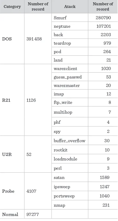
The KDD 99 dataset has around two million connection records in the two weeks of test. Each connection is labeled as either normal, or as an attack, with exactly one specific attack type, and contains 41 features (such as duration, protocol type, service, flag, source bytes, ...). Attacks fall into four main categories: DOS (denial of service), R2L (unauthorized access from a remote machine), U2R (unauthorized access to local superuser (root) privileges), and probing (surveillance and other probing) [18].

At the International Knowledge Discovery and Data Mining Tools Competition (IKDDMTC), “10% KDD 99” dataset is employed for the purpose of training. The attack categories along with the number of records that were attacked are listed in Table 2.

Table 210% KDD 99 intrusion detection dataset [18] 4.1. Feature Dataset

The KDD 99 dataset has around two million connec-tion records in the two weeks of test. Each connecconnec-tion is labeled as either normal, or as an attack, with exact-ly one specific attack type, and contains 41 features (such as duration, protocol type, service, flag, source bytes, ...). Attacks fall into four main categories: DOS (denial of service), R2L (unauthorized access from a remote machine), U2R (unauthorized access to local superuser (root) privileges), and probing (surveil-lance and other probing) [18].

At the International Knowledge Discovery and Data

(7)

Table 2

10% KDD 99 intrusion detection dataset [18]

Category Number of _record Atack Number of _record

DOS 391 458

Smurf 280790 neptune 107201

back 2203

teardrop 979

pod 264

land 21

R21 1126

warezclient 1020 guess_passwd 53 warezmaster 20

imap 12

ftp_write 8 multihop 7

phf 4

spy 2

U2R 52

buffer_overflow 30 rootkit 10 loadmodule 9

perl 3

Probe 4107

satan 1589 ipsweep 1247 portsweep 1040

nmap 231

Normal 97277

4.2. Fast Independent Component Analysis (ICA)

Fast adaptive ICA algorithm is used in this paper in order to extract independent components of sampled data. ICA attempts to decompose a multivariate sig-nal into independent non-Gaussian sigsig-nals. ICA has been considered as a fundamental tool in the field of data analysis, feature extraction, and so on. The KDD 99 intrusion detection database includes non-Gauss-ian distribution, so ICA techniques are suitable for feature extraction in this field. Feature reduction plays an important role in case of improving ID per-formance and reducing the computational complexi-ty, especially in an online detection.

The detailed formulation of FastAdaptiveOgICA is given in [41]. Not only is this method fast and adap-tive with iteraadap-tive neural network algorithm, it can also instantly separate mixture of sub-Gaussian and super-Gaussian signals. It has fast convergence speed and high separation performance.

Dimension reduction reduces the complexity of the proposed IDS significantly leading to less computa-tional complexity and also fast and accurate intru-sion detection. Implementation of fast adaptive ICA algorithm on the distinct KDD sample set leads to extraction of independent component of the dataset, and as a result, a new dataset with fewer dimensions is constructed. The new dataset is then used for neu-ral network training in order to obtain Instantaneous Firing Speeds (IFSs) and the arc weights of the pro-posed FOHPN models. Table 4 shows the number of records before ICA and after implementing fast adap-tive ICA algorithm.

Category Normal Probe U2R R2L DOS Distinct

Train

Records 2996 11656 52 995 45927

Distinct Test

Records 9711 1106 37 2199 5741

Table 3

Number of distinct records in the KDD train set

Table 4

Number of data after implementing fast adaptive ICA algorithm in each category

Category Normal Probe U2R R2L DOS Dimension

before ICA 2996 11656 52 995 45927

Reduced

dimension 138 132 30 86 138

4.3. Proposed Neural FOHPN

(8)

models have been considered by some researchers in the late 90’s [9, 2]. A viable approach to detect cyber threats in CPSs appears to be neural FOHPN, since CPSs are event driven systems comprised of both dis-crete event and continuous dynamics. This is, in fact, the approach that is proposed in this paper.

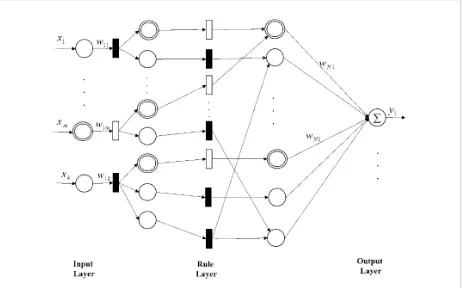
4.3.1. Feedforward Neural FOHPN Architecture For the purpose of anomaly detection, the FOHPN network shown in Fig. 8 consisting of the following three layers: input layer, rule layer, and output layer, are considered.

Define tj as the set of transitions of the jth layer of the neural FOHPN, which the corresponding weights are assumed to be _{w w}₁j, ,...,₂j _wj

η. In the sequel, first the

formulation for the discrete transitions is approved. The net dynamic of FOHPN varies when a macro event occurs. In this situation, a discrete transition fires. This may change the discrete marking or en-abling/disabling a continuous transition.

In the proposed model, when a discrete transition be-comes firable, it just may change the marking of dis-crete transitions. Let

σ κ

( ) be the firing count vector at time instant

κ

. The macro-behavior of the FOHPN is defined during the

κ

th macro-period by [7]:

( 1) = ( ) . ( 1), ( 1) = ( ).

d d c c

dd

m κ+ m κ +C σ κ+ m κ+ m κ

( 1) = ( ) . ( 1), ( 1) = ( ).

d d c c

dd

m κ+ m κ +C σ κ+ m κ+ m κ (2)

The output of the jth layer can be written as:

=1

= = ( ) ,

j T j j

i i i

X W M

∑

ηm p w

( ) = ( ) = (j j T ),

Y X F X F W M

where m is the marking of the net as defined in (2). Now, the learning algorithm formulation in the rule layer is presented. Here, the back propagation meth-od, which is the most common training method for

Figure 8

Framework of neural FOHPN

Fig. 8.Framework of neural FOHPN

We consider a neural FOHPN model having k rule layers. We therefore have a total of k+2 layers including input and output layers that are numbered as 0,...,k+1.

The number of input and output places are r and L, respectively. There exist N places in the hidden layers. The training data for a feedforward network consist of q input-output data pairs. n denotes training instance. So, we define the input vector X _{and the output vector}_Y _{as follows:}

1

( ) = [ ( ),..., ( )] ,T k X n x n x n

1 1

1

( ) = [ k ( ),..., k ( )] ,T L Y n y+ n y+ n

Therefore, for the jth layer one can write:

1

=1,...,

( ) = ( . ( ))

j j

i i

j N

y n F w x nβ β β

+

∑

₍₃₎

1 1

1

(9)

feedforward networks, is used. Useful information about neural network and recurrent neural network is invoked from [19].

We consider a neural FOHPN model having k rule layers. We therefore have a total of k + 2 layers in-cluding input and output layers that are numbered as 0, ..., k + 1.

The number of input and output places are r and L, re-spectively. There exist N places in the hidden layers. The training data for a feedforward network consist of q input-output data pairs. n denotes training in-stance. So, we define the input vector X ˚ and the out-put vector Y as follows:

1

( ) = [ ( ),..., ( )] ,T k X n x n x n

1 1

1

( ) = [ k ( ),..., k ( )] ,T L Y n y + n y + n

Therefore, for the jth layer one can write:

1 =1,..., ( ) = ( . ( )) j j i i j N

y n F w x nβ β

β

+

∑

1 1

1

( ) = [ k ( ),..., k ( )] ,T L Y n y + n y + n

(3)

where w_iβ is the arc weight between i and

β

places

in different layers. In order to find the arc weights of the network, an optimization problem must be solved. The following summed square error is considered as an objective function:

2

=1,..., =1,...,

= ( ) ( ) = ( ).

n q n q

E

∑

Y n Y n-

∑

E n ₍₄₎

Minimization of the cost function is done using gra-dient concept: =1,..., ( ) = . j j t q i i

E E n

wβ wβ

∂ ∂

∂

∑

∂

By using a small learning rate γ, one can write:

( )

( 1) = ( ) .

j j

i i j

i E n w w w β β β

w

+

w γ

- ∂

∂

All training samples are used to update the new weights. One such pass through all samples is called

an epoch. Arc weights should be initialized, typically to small random numbers, before the first epoch. The gradient ( )_j

i E n

wβ ∂

∂ can be computed as follows:

( )₌ ( )_* ( ) ( )

j j

i i

E n E n Y n

wβ Y n wβ

∂ ∂ ∂

=1,...,

( ) = ( ) ( ) * jj * jj.

n q i

F X X

Y n Y n

X wβ

∂ ∂

-∂ ∂

∑

To each discrete transitions t T_i∈ _D in FOHPN, we as-sign an average firing rate

λ

_i= ( )D t_i for an exponen-tially distributed timed transition t T_i∈ _E, hence:

( ) =

1 exp( ( ))

j j

j j j

F X

X b X

μ

λ

∂

∂ + -

-2

*exp( ( _{)) ,} [1 exp( ( ))]

j j j j

j j

X b b X

b X

μ

λ

- -+ + - -= ( ). j j i j i

X _{m p}

wβ

∂ ∂

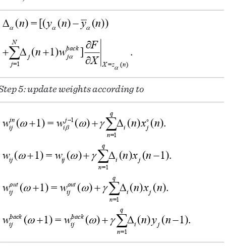
Afterward, the iterative Algorithm 1 is proposed to minimize the error using back propagation method in each epoch for the discrete net of the proposed neural FOHPN model:

Algorithm 1:

Step 0: set ω = 0, ρ = P (ρ is a predetermined maximal number of epochs), and error = ε.

Step 1: initialize weights to some small random num-bers.

Step 2: for each sample n, compute intermediate layers outputs, except for input layer, from (3).

Step 3: compute error propagation term of the output layer

( ) j i n

Δ backward through j = k + 1, k,...,1.

1

1 =

( ) = [ ( ) ( )]

k

i i i

k X zi F

n y n y n

X + + ∂ Δ -∂ ,

where 1 1 1

=1

( ) = ( )

j N

j j j

i i

z n xα n wα

α

--

-∑

.

(10)

1 1 =1 = ( ) = j N

j j j

i i m X zi F n w X ϕ ϕ ϕ + + ∂ Δ Δ ∂

∑

.

Step 5: update the weights according to

1 1 1

=1

( 1) = ( ) q ( ) ( ).

j j j j

i i i

n

wβ-

w

+ wβ-

w γ

+

∑

Δ n xβ- n

Step 6: after each epoch, error should be computed

based on (4). If error >ε, or ω < P, then set ω = ω +1 and go to step 1; else go to step 7.

Step 7: End.

Subsequently, the same formulation for continuous transitions of the proposed neural FOHPN model will be derived. The whole framework of the new formu-lation is similar to previous one with the following differences.

The IFS of time transition ti∈ Tc is denoted by vi( )τ .

The marking of a place p ∈ Pc is represented by

( ) = ( ) . ( ) ( ), m

τ

+d

τ

m

τ

+w v d

τ

( ) _{( ) = . ( ).} ( )

m d m _{w v}

d

τ

_τ

τ

+

-It is assumed that at time τ, no discrete transition is fired and all speeds are continuous. So, we have:

( ) = ( , ). ( ).i i t T_{i c}

dm _{C p t v}

d

τ

_τ

τ

∑

∈ (5)

A macro-event occurs by firing of a discrete transition or when a continuous place becomes empty. Firing of a discrete transition changes the discrete marking or enables/disables a continuous transition. The en-abling state of a continuous transition changes from strong to weak, when a continuous place becomes empty. Let

τ τ

_k

,

_k₊₁ be the occurrence times of mac-ro-events; the time interval is called macro-period. Furthermore, it is assumed that during a macro-pe-riod the IFS of continuous transitions are constant, and

τ

₀ is the initial time,

τ

_k( > 0)k is the instants in which macro-events occur, and v( )

τ

k is the IFS vec-tor during the macro-period of length Δ_k. The mac-ro-behavior of an FOHPN during the kth macro-peri-od is defined as follows [7]:

( ) = ( ) . ( ).( ), ( ) = ( ).

c c d d

k cc k k k

m τ m τ +C vτ τ τ- m τ m τ

( ) = ( ) . ( ).( ), ( ) = ( ).

c c d d

k cc k k k

m τ m τ +C vτ τ τ- m τ m τ (6)

In this case, the jth layer output of the FOHPN can be written as

( ) = ( ) = (j j T ),

Y X F X F W M

where M is continuous marking defined by (6), and F= v(t). The rest of the formulation is the same as pre-viously proposed algorithm for discrete net and can be derived directly.

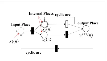
A typical time delay neural FOHPN is implemented as a feedforward neural FOHPN. It has three layers as introduced: input, hidden and output layers. Just a set of delays are added to the inputs. Time delay can be easily implemented in the PN by considering delay in the firing time of the transitions. Time delay neural FOHPN is applied in order to detect anomaly and the performance comparison is provided in Section 4.4. 4.3.2. Recurrent Neural FOHPN Architecture Recurrent neural network has lots of similarities with feedforward neural network, but in the former struc-ture, at least one cyclic path exists. Since cyclic path can easily be incorporated by FOHPN model, the re-current neural network structure can be applied in or-der to update the weights in the FOHPN. Fig. 9 shows a simple recurrent neural network FOHPN structure. This net with two cyclic arcs has one input place, two hidden places, and one output place.

Suppose that the recurrent neural FOHPN model has k input, N internal, and L output places represented by

Figure 9

An example of FOHPN with recurrent structure ( ) = ( ) = (j j T ), Y X F X F W M

where M is continuous marking defined by (6), and F v t= ( ). The rest of the formulation is the same as previously proposed algorithm for discrete net and can be derived directly.

A typical time delay neural FOHPN is implemented as a feedforward neural FOHPN. It has three layers as introduced: input, hidden and output layers. Just a set of delays are added to the inputs. Time delay can be easily implemented in the PN by considering delay in the firing time of the transitions. Time delay neural FOHPN is applied in order to detect anomaly and the performance comparison is provided in Section 4.4.

4.3.2 Recurrent Neural FOHPN Architecture

Recurrent neural network has lots of similarities with feedforward neural network, but in the former structure, at least one cyclic path exists. Since cyclic path can easily be incorporated by FOHPN model, the recurrent neural network structure can be applied in order to update the weights in the FOHPN. Fig. 9 shows a simple recurrent neural network FOHPN structure. This net with two cyclic arcs has one input place, two hidden places, and one output place.

Fig. 9.An example of FOHPN with recurrent structure

Suppose that the recurrent neural FOHPN model has k input, N internal, and L output places represented by X n( ) = [ ( ),..., ( )] ,x n1 x nk T X n( ) = [ ( ),..., ( )] ,x n1 x nN T Y n( ) = [y1k+1( ),...,n yLk+1( )]n T , respectively. Furthermore, let _{W W W W}in, , out, back _{be input}₍_{N K}_× _), _internal ₍_{N N}_× ₎ _{, output}

(L K N×( + )), and back projection (N L× ) connection weight matrices; respectively. _Fout _{indicates a} given activation function of the output layer. As a whole structure, we have:

( 1) = ( in ( 1) ( ) back ( )) X n+ F W X n + +WX n W Y n+

(

)

(

)

( 1) = out out ( 1), ( 1) . Y n+ F W X n + X n+

(11)

1

( ) = [ ( ),..., ( )] ,T k X n x n x n

1

( ) = [ ( ),..., ( )] ,T N X n x n x n

1 1

1

( ) = [ k ( ),..., k ( )]T L

Y n y + n y + n _{, respectively.} Further-more, let _{W W W W}in, , out, back_{be input}₍_{N K}_× _), in-ternal (N N× ), output (L K N×( + )), and back projection (N L× ) connection weight matrices; re-spectively. _Fout_{indicates a given activation function} of the output layer. As a whole structure, we have:

( 1) = ( in ( 1) ( ) back ( ))

X n+ F W X n + +WX n W Y n+

(

)

(

)

( 1) = out out ( 1), ( 1) .

Y n+ F W X n + X n+

Discrete and continuous marking are the same as (1) and (5). Activation function F was defined for two cases of macro events occurrence. Back propagation algorithm is applied in the rule layer. The learning procedure is the same as previous one, but a new algo-rithm (based on [19]) must be proposed to iteratively update the weights:

Algorithm 2

Step 0: set ω = 0, ρ = P (ρ is a predetermined maximal number of epochs), and error = ε.

Step 1: first of all, weights should be initialized to small random numbers.

Step 2: for forward path, weights can be computed based on Algorithm 1.

Step 3: compute error propagation term of the output layer Δ_i(n) by proceeding backward through n = q,...,1, for each sample n:

=1 = ( )

( ) = [ [ ( )L ( )]

i i i

j X z q_i

F

q y q y q

X ∂ Δ -∂

∑

= ( )

* out] .

ji

X z n_i F w

X

∂ ∂

Step 4: compute error propagation term of the rule lay-ers as follows:

=1

( ) = [N ( 1)

i n α n wαi

α

Δ

∑

Δ +

=1 = ( )

( ) ] .

L

out i

X z n_i F n w X α α α ∂ + Δ ∂

∑

where,

( ) = [( ( )n y n y n( ))

α α α

Δ

-=1 = ( )

( 1) ] .

N

back

j j

j X z n

F n w X α α ∂ + Δ + ∂

∑

Step 5: update weights according to

1

=1

( 1) = ( ) ( ) ( ).

( 1) = ( ) ( ) ( 1).

( 1) = ( ) ( ) ( ).

( 1) = ( ) ( ) ( 1).

q

in j

ij i i j

n q

ij ij i j

n q

out out

ij ij i j

n q

back back

ij ij i j

n

w w n x n

w w n y n

β

w

w γ

w

w γ

w

w γ

w

w γ

-+ + Δ + + Δ -+ + Δ + + Δ

-∑

∑



Step 6: after each epoch, error should be comput-ed bascomput-ed on (4) if If error > ε, or ω < P or . Then, set ω = ω +1 , and go to step 1;else go to step 7.

Step 7: End.

4.4. Validation of the Approach and Simulation Results

Using the proposed feedforward neural FOHPN, time delay neural FOHPN, and recurrent neural FOHPN, three novel models were introduced for anomaly de-tection in CPSs. Measured features in KDD 99 dataset are defined as the initial conditions of the input plac-es in the proposed models. A complete list of featurplac-es defined for the connection records is given in Table 5. As can be seen, some features of KDD 99 intrusion detection dataset are continuous and some are dis-crete. Consequently, the FOHPN is proposed in order to capture both feature types. All 41 features listed in Table 5 are used as the initial marking of the proposed neural FOHPN models. Based on the previously pro-posed training algorithms, appropriate unknown pa-rameters such as arc weights, firing speeds, and time delays can be computed. After the training procedure, these parameters are set in the proposed models, and validation is done based on the test dataset.

(12)

at-231 Information Technology and Control 2018/2/47

Table 5

Basic features of KDD 99 intrusion detection dataset [18]

tacks in the CPSs, three different methods, namely feedforward back propagation neural FOHPN, time delay neural FOHPN, and recurrent neural FOHPN have been used. Each model leads to a different

(13)

A comparison of detection rate (DR) for the DARPA test dataset using the proposed models is presented in Table 7.

Figure 10

Performance evaluation of the (a) feedforward back propagation neural FOHPN, (b) recurrent neural FOHPN, (c) time delay neural FOHPN

Table 6

Performance comparison of the proposed neural FOHPN models

Running _{time (s)} Accuracy (norm _{of error)}

Feedforward back

propagation neural FOHPN 6 0.470

Recurrent neural FOHPN 149 0.224

time delay neural FOHPN 48 0.332

Fig. 10

Performance evaluation of the (a) feedforward back propagation neural FOHPN, (b) recurrent

neural FOHPN, (c) time delay neural FOHPN

A comparison of detection rate (DR) for the DARPA test dataset using the proposed models is presented

in Table 7.

Table 6

Performance comparison of the proposed neural FOHPN models

Running time (s) Accuracy (norm of error) Feedforward back propagation neural FOHPN 6 0.470

Recurrent neural FOHPN 149 0.224 time delay neural FOHPN 48 0.332

Table 7

Detection rate comparison of the proposed FOHPN models

Normal Dos Probe U2R R2L Feedforward back propagation neural FOHPN 98.2 99.8 99.5 99.0 96.2 Recurrent neural FOHPN 97.9 99.4 98.7 98.5 94.0 Time delay neural FOHPN 99.2 98.5 99.2 98.9 96.0

Based on these results, all three models are accurate enough, but the running time of feedforward back

propagation neural FOHPN is considerably smaller than others. Since the time of cyber detection is

Fig. 10

Performance evaluation of the (a) feedforward back propagation neural FOHPN, (b) recurrent

neural FOHPN, (c) time delay neural FOHPN

A comparison of detection rate (DR) for the DARPA test dataset using the proposed models is presented

in Table 7.

Table 6

Performance comparison of the proposed neural FOHPN models

Table 7

Detection rate comparison of the proposed FOHPN models

Based on these results, all three models are accurate enough, but the running time of feedforward back

propagation neural FOHPN is considerably smaller than others. Since the time of cyber detection is

Fig. 10

Performance evaluation of the (a) feedforward back propagation neural FOHPN, (b) recurrent

neural FOHPN, (c) time delay neural FOHPN

A comparison of detection rate (DR) for the DARPA test dataset using the proposed models is presented

in Table 7.

Table 6

Performance comparison of the proposed neural FOHPN models

Table 7

Detection rate comparison of the proposed FOHPN models

Based on these results, all three models are accurate enough, but the running time of feedforward back

propagation neural FOHPN is considerably smaller than others. Since the time of cyber detection is

a

b

c

Table 7

Detection rate comparison of the proposed FOHPN models

Normal Dos Probe U2R R2L

Feedforward back propagation

neural FOHPN 98.2 99.8 99.5 99.0 96.2

Recurrent neural

FOHPN 97.9 99.4 98.7 98.5 94.0

Time delay neural

FOHPN 99.2 98.5 99.2 98.9 96.0

Figure 11

Anomaly detection error based on feedforward neural FOHPN model

critically important, feedforward back propagation neural FOHPN seems to be more useful. Fig. 11 indicates anomaly detection errors based on feedforward neural FOHPN in all four attack categories and normal condition. As can be seen, the error on the test dataset is driven to a very small value.

Fig. 11Anomaly detection error based on feedforward neural FOHPN model

To verify the effectiveness of the proposed model against existing neural-network-based approaches, a performance comparison of detection rate (DR) and false positive rate (FPR)1_{is provided in Table 8. All}

methods are implemented using MATLAB toolbox in the same PC.

Based on the result shown in Table 8, it is evident that the proposed feedforward back propagation neural FOHPN model is accurate enough to enhance acceptable detection rate. Its accuracy is better than [14], [42], and [20], and fairly close to [29], however, its running time is much smaller than the others. This factor is very critical in cyber intrusion detection concept. The speed of the proposed method is 13 times faster than the fastest one. As a result, one can conclude that not only feedforward back propagation neural FOHPN is satisfactorily accurate, but also the required time to detect abnormal or malicious behavior is much less than other methods. This efficiency is indeed expected based on Petri net properties.

Table 8Performance comparison of the proposed FOHPN model with other approaches

Normal Dos Probe U2R R2L Running DR FPR DR FPR DR FPR DR FPR DR FPR Time (s) feedforward back

propagation neural FOHPN 98.2 2.9 100 1.6 99.5 1.2 99 0.6 96.2 0.4 0.1228 BPNN [14] 79.8 - 97.5 - 99.1 - 34.5 - 98.9 - 2.5 RBF [42] - - 98.8 1.6 98 1.6 - - 97.2 1.6 1.6 HPCANN [29] - - 100 0.7 100 0.5 - - 97.2 0.6 -MLP [20]

- - 99.9 - 48.1 - 48.3 - 93.2 - 30

(14)

Table 8

Performance comparison of the proposed FOHPN model with other approaches

Normal Dos Probe U2R R2L Running

DR FPR DR FPR DR FPR DR FPR DR FPR Time (s)

Feedforward back propagation neural

FOHPN 98.2 2.9 100 1.6 99.5 1.2 99 0.6 96.2 0.4 0.1228

BPNN [14] 79.8 - 97.5 - 99.1 - 34.5 - 98.9 - 2.5

RBF [42] - - 98.8 1.6 98 1.6 - - 97.2 1.6 1.6

HPCANN [29] - - 100 0.7 100 0.5 - - 97.2 0.6

-MLP [20] -- -- 99.9 -- 48.1 -- 48.3 -- 93.2 -- 30

Based on these results, all three models are accurate enough, but the running time of feedforward back propagation neural FOHPN is considerably smaller than others. Since the time of cyber detection is crit-ically important, feedforward back propagation neu-ral FOHPN seems to be more useful. Fig. 11 indicates anomaly detection errors based on feedforward neu-ral FOHPN in all four attack categories and normal condition. As can be seen, the error on the test dataset is driven to a very small value.

To verify the effectiveness of the proposed model against existing neural-network-based approaches, a performance comparison of detection rate (DR) and false positive rate (FPR)1_{is provided in Table 8. All}

methods are implemented using MATLAB toolbox in the same PC.

Based on the result shown in Table 8, it is evident that the proposed feedforward back propagation neural FOHPN model is accurate enough to enhance acceptable detection rate. Its accuracy is better than [14], [42], and [20], and fairly close to [29], howev-er, its running time is much smaller than the others. This factor is very critical in cyber intrusion detec-tion concept. The speed of the proposed method is 13 times faster than the fastest one. As a result, one can conclude that not only feedforward back prop-agation neural FOHPN is satisfactorily accurate, but also the required time to detect abnormal or

ma-1 It occurs when it is normal while IDS detects it attack.

licious behavior is much less than other methods. This efficiency is indeed expected based on Petri net properties.

5. Conclusion

(15)

References

1. Abbes, T., Bouhoula, A. Rusinowitch, M. Protocol Analysis in Intrusion Detection Using Decision Tree. International Conference on Information Technolo-gy: Coding and Computing, 2004. Proceedings. ITCC 2004, 2004, 1, 404-408. https://doi.org/10.1109/ ITCC.2004.1286488

2. Ahson, S. I. Petri Net Models of Fuzzy Neural Networks. IEEE Transactions on Systems, Man, and Cybernetics, 1995, 25(6), 926-932. https://doi.org/10.1109/21.384255 3. Alarcon-Aquino, V., Ramirez-Cortes, J. M., Gomez-Gil,

P., Starostenko, O. Garcia-Gonzalez, Y. Network Intru-sion Detection Using Self-Recurrent Wavelet Neural Network with Multidimensional Radial Wavelons. In-formation Technology and Control, 2014, 43(4), 347-358. https://doi.org/10.5755/j01.itc.43.4.4626

4. Anderson, D., Frivold, T. Valdes, A. Next-Generation In-trusion Detection Expert System (Nides): A Summary, 1995.

5. Anderson, J. P. Computer Security Threat Monitoring and Surveillance. Technical Report, James P. Anderson Company, 1980.

6. Antonatos, S., Anagnostakis, K. G. Markatos, E. P. Gen-erating Realistic Workloads for Network Intrusion Detection Systems. ACM SIGSOFT Software Engi-neering Notes, ACM, 2004, 29, 207-215. https://doi. org/10.1145/974043.974078

7. Balduzzi, F., Giua, A. Menga, G. First-Order Hybrid Pe-tri Nets: A Model for Optimization and Control. IEEE Transactions on Robotics and Automation, 2000, 16(4), 382-399. https://doi.org/10.1109/70.864231

8. Bitter, C., North, J., Elizondo, D. A., Watson, T. An In-troduction to the Use of Neural Networks for Network Intrusion Detection. Computational Intelligence for Privacy and Security, Springer, 2012, 5-24.

9. Chow, T. W., Li, J.-Y. Higher-Order Petri Net Models Based on Artificial Neural Networks. Artificial Intelli-gence, 1997, 92(1-2), 289-300. https://doi.org/10.1016/ S0004-3702(96)00048-3

10. Chung, Y. Y., Wahid, N. A Hybrid Network Intrusion Detection System Using Simplified Swarm Optimiza-tion (SSO). Applied Soft Computing, 2012, 12(9), 3014-3022. https://doi.org/10.1016/j.asoc.2012.04.020 11. Denatious, D. K., John, A. Survey on Data Mining

Tech-niques to Enhance Intrusion Detection. IEEE Interna-tional Conference on Computer Communication and

Informatics (ICCCI), 2012, 1-5. https://doi.org/10.1109/ ICCCI.2012.6158822

12. Dolgikh, A., Nykodym, T., Skormin, V., Antonakos, J., Baimukhamedov, M. Colored Petri Nets as the En-abling Technology in Intrusion Detection Systems. IEEE Military Communications Conference MIL-COM, 2011, 1297-1301. https://doi.org/10.1109/MIL-COM.2011.6127481

13. Goyal, M. K., Aggarwal, A. Composing Signatures for Misuse Intrusion Detection System Using Genetic Al-gorithm in an Offline Environment. Advances in Com-puting and Information Technology, Springer, 2012, 151-157.

14. Haddadi, F., Khanchi, S., Shetabi, M., Derhami, V. In-trusion Detection and Attack Classification Using Feed-Forward Neural Network. IEEE Second Interna-tional Conference on Computer and Network Technol-ogy (ICCNT), 2010, 262-266. https://doi.org/10.1109/ ICCNT.2010.28

15. Han, S., Xie, M., Chen, H.-H., Ling, Y. Intrusion Detec-tion in Cyber-Physical Systems: Techniques and Chal-lenges. IEEE Systems Journal, 2014, 8(4), 1052-1062. https://doi.org/10.1109/JSYST.2013.2257594

16. Helmer, G., Wong, J., Slagell, M., Honavar, V., Miller, L., Wang, Y., Wang, X., Stakhanova, N. Software Fault Tree and Coloured Petri Net–Based Specification, Design and Implementation of Agent-Based Intrusion Detec-tion Systems. InternaDetec-tional Journal of InformaDetec-tion and Computer Security, 2007, 1(1-2), 109-142. https://doi. org/10.1504/IJICS.2007.012246

17. Horng, S. J., Su, M. Y., Chen, Y. H., Kao, T. W., Chen, R. J., Lai, J. L., Perkasa, C. D. A Novel Intrusion Detection System Based on Hierarchical Clustering and Sup-port Vector Machines. Expert Systems with Applica-tions, 2011, 38(1), 306-313. https://doi.org/10.1016/j. eswa.2010.06.066

18. KDD Cup 1999 Data. Available at http://kdd.ics.uci.edu/ databases/kddcup99/kddcup99.html.

19. Jaeger, H. Tutorial on Training Recurrent Neural Net-works, Covering BPPT, RTRL, EKF and the” Echo State Network” Approach, 2002, 5.

(16)

21. Kim, G., Lee, S., Kim, S. A Novel Hybrid Intrusion De-tection Method Integrating Anomaly DeDe-tection with Misuse Detection. Expert Systems with Applications, 2014, 41(4), 1690-1700. https://doi.org/10.1016/j. eswa.2013.08.066

22. Kshirsagar, V. K., Tidke, S. M., Vishnu, S. Intrusion Detec-tion System Using Genetic Algorithm and Data Mining: An Overview. International Journal of Computer Sci-ence and Informatics ISSN (PRINT), 2012, 2231, 5292. 23. Kumar, S. Classification and Detection of Computer

In-trusions. Ph.D. thesis, Purdue University, 1995.

24. Lee, W., Stolfo, S. J., Mok, K. W. Mining Audit Data to Build Intrusion Detection Models. KDD, 1998, 66-72. 25. Lei, J. Z., Ghorbani, A. A. Improved Competitive

Learn-ing Neural Networks for Network Intrusion and Fraud Detection. Neurocomputing, 2012, 75(1), 135-145. https://doi.org/10.1016/j.neucom.2011.02.021

26. Li, W. Using Genetic Algorithm for Network Intrusion Detection. Proceedings of the United States Depart-ment of Energy Cyber Security Group, 2004, 1, 1-8. 27. Li, Y., Wang, Y. A Misuse Intrusion Detection Model

Based on Hybrid Classifier Algorithm. International Journal of Digital Content Technology and Its Applica-tions, 2012, 6(5), 352-365.

28. Liao, H.-J., Lin, C.-H. R., Lin, Y.-C., Tung, K.-Y. Intrusion detection System: A Comprehensive Review. Journal of Network and Computer Applications, 2013, 36(1), 16-24. https://doi.org/10.1016/j.jnca.2012.09.004

29. Liu, G., Yi, Z., Yang, S. A Hierarchical Intrusion Detec-tion Model Based on the PCA Neural Networks. Neu-rocomputing, 2007, 70(7-9), 1561-1568. https://doi. org/10.1016/j.neucom.2006.10.146

30. McHugh, J. Intrusion and Intrusion Detection. Interna-tional Journal of Information Security, 2001, 1(1), 14-35. https://doi.org/10.1007/s102070100001

31. Mitchell, R., Chen, I.-R. A Survey of Intrusion Detection Techniques for Cyber-Physical Systems. ACM Com-puting Surveys (CSUR), 2014, 46(4), 55(1-29).

32. Mitchell, R., Chen, R. Behavior-Rule Based Intrusion Detection Systems for Safety Critical Smart Grid Appli-cations. IEEE Transactions on Smart Grid, 2013, 4(3), 1254-1263. https://doi.org/10.1109/TSG.2013.2258948 33. Modi, C., Patel, D., Borisaniya, B., Patel, H., Patel, A.,

Rajarajan, M. A Survey of Intrusion Detection

Tech-niques in Cloud. Journal of Network and Computer Ap-plications, 2013, 36(1), 42-57. https://doi.org/10.1016/j. jnca.2012.05.003

34. Morris, T. H., Srivastava, A. K., Reaves, B., Pavurapu, K., Abdelwahed, S., Vaughn, R., McGrew, W., Dandass, Y. Engineering Future Cyber-Physical Energy Sys-tems: Challenges, Research Needs, and Roadmap. IEEE North American Power Symposium (NAPS), 2009, 1-6. https://doi.org/10.1109/NAPS.2009.5484019

35. Muda, Z., Yassin, W., Sulaiman, M., Udzir, N. Intrusion Detection Based on K-Means Clustering and Naive Bayes Classification. IEEE 7th International Confer-ence on Information Technology in Asia (CITA 11), 2011, 1-6.

36. Raciti, M. Anomaly Detection and Its Adaptation: Stud-ies on Cyber-Physical Systems. Ph.D. thesis, Linköping University Electronic Press, 2013.

37. Srinivasu, P., Avadhani, P. Genetic Algorithm Based Weight Extraction Algorithm for Artificial Neural Net-work Classifier in Intrusion Detection. Procedia En-gineering, 2012, 38, 144-153. https://doi.org/10.1016/j. proeng.2012.06.021

38. Tavallaee, M., Bagheri, E., Lu, W., Ghorbani, A. A. A Detailed Analysis of the KDD Cup 99 Data Set. IEEE Symposium on Computational Intelligence for Secu-rity and Defense Applications, 2009, 1-6. https://doi. org/10.1109/CISDA.2009.5356528

39. Wang, G., Hao, J., Ma, J., Huang, L. A New Approach to intrusion Detection Using Artificial Neural Networks and Fuzzy Clustering. Expert Systems with Applica-tions, 2010, 37(9), 6225-6232. https://doi.org/10.1016/j. eswa.2010.02.102

40. Xu, Y.-Q., Zhang, B., Qin, X.-T. Clustering Intrusion De-tection Model Based on Grey Fuzzy K-Mean Clustering. Journal of Chongqing Normal University (Natural Sci-ence), 2013, 1, 0-19.

41. Ye, Y., Zhang, Z.-L., Zeng, J., Peng, L. A Fast and Adaptive ICA Algorithm with Its Application to Fetal Electrocar-diogram Extraction. Applied Mathematics and Compu-tation, 2008, 205(2), 799-806. https://doi.org/10.1016/j. amc.2008.05.117