Separator-Based Pruned Dynamic Programming for Steiner Tree

The Thirty-Third AAAI Conference on Artificial Intelligence (AAAI-19)

Separator-Based Pruned Dynamic Programming for Steiner Tree

Yoichi Iwata

[email protected]

Takuto Shigemura

Abstract

Steiner tree is a classical NP-hard problem that has been ex-tensively studied both theoretically and empirically. In theory, the fastest approach for inputs with a small number of termi-nals uses the dynamic programming, but in practice, state-of-the-art solvers are based on the branch-and-cut method. In this paper, we present a novel separator-based pruning tech-nique for speeding up a theoretically fast DP algorithm. Our empirical evaluation shows that our pruned DP algorithm is quite effective against real-world instances admitting small separators, scales to more than a hundred terminals, and is competitive with a branch-and-cut solver.

Introduction

For an undirected graphG= (V, E)and a terminal setA⊆

V, a tree inGis called aSteiner treeif it connects all the terminals inA. An input to the Steiner tree problem is an undirected graphG= (V, E)with an edge-weight function w : E → R>0 and a terminal setA ⊆ V, and the task is

to find a Steiner tree with the minimum total weight. We use n,m, and k to denote the number of vertices, edges, and terminals, respectively.

The Steiner tree problem has been extensively studied both theoretically and empirically. In theoretical studies, Steiner tree is known as one of the Karp’s 21 NP-complete problems and has been studied from various theoretical viewpoints including approximation algorithms and fixed-parameter-tractable algorithms. In empirical studies, Steiner tree is known to have many applications in various fields in-cluding the VLSI design of microchips (Held et al. 2011), the design of fiber-optic networks (Leitner et al. 2014), key-word search in relational databases (Ding et al. 2007), and team formulation in social networks (Lappas, Liu, and Terzi 2009)1. Due to its practical importance, in recent years, two Copyright c2019, Association for the Advancement of Artificial Intelligence (www.aaai.org). All rights reserved.

1_{The latter two applications use the following variant of Steiner} tree, calledgroup Steiner tree: given a set of groups of vertices in-stead of the terminals, find a minimum-weight connected tree con-taining at least one vertex from each group. We can solve this vari-ant by a reduction to the standard Steiner tree (for details, see, e.g., (Zachariasen and Rohe 2003) or (Gamrath et al. 2017)). Actually, the datasets we use in the experiments contain instances obtained by this reduction.

competitions of Steiner tree solvers, the 11th DIMACS Im-plementation Challenge (2014) and the 3rd Parameterized Algorithms and Computational Experiments (PACE) Chal-lenge (2018), were held, and development of practically fast Steiner tree solvers has attracted a lot of attention.

In theory, the Steiner tree problem is known to be fixed parameter tractable (FPT)parameterized by the number of terminalsk; i.e., it can be solved in f(k)poly(n)time for some computable functionf. This means that, although the problem is NP-hard in general, it is easy when the number of terminals is small. The first FPT algorithm was obtained by Dreyfus and Wagner (Dreyfus and Wagner 1971) and has a time complexityO(3k_{nm). This algorithm has been} improved in two directions: in terms of thepoly(n)factor, the current fastest FPT algorithm runs inO(3k_{n+ 2}k_(m+ nlogn)) time (Erickson, Monma, and Veinott 1987), and in terms of the f(k)factor, the current fastest one runs in

O((2 +)k_ng()_{)time for any > 0for some functiong}

(Fuchs et al. 2007).

All of these FPT algorithms solve the problem as follows. LetT be a minimum Steiner tree for terminalsAand pick a terminalu∈A. Ifuhas degree one inT,T is the union of the unique incident edgeuvand the minimum Steiner tree for terminals(A\ {u})∪ {v}. Ifuhas degree at least two, T is the union of the minimum Steiner tree for A1∪ {u}

and the minimum Steiner tree forA2∪ {u}for some

parti-tionA=A1∪A2∪ {u}. Conversely, any minimum Steiner

tree can be obtained by recursively applying these two op-erations, and therefore, we can solve the problem by com-puting a minimum Steiner tree for terminals S∪ {u} for every subsetS ⊆ Aand every vertexu ∈ V in a bottom-up from small to large by using the dynamic programming (DP). This is why the dependence on k is exponential. It has been theoretically proved that avoiding the exponential dependence onk is difficult; under the Set Cover Conjec-ture, the Steiner tree withk terminals cannot be solved in (2−)kpoly(n)time for any > 0 (Cygan et al. 2016), and under the Exponential-Time Hypothesis, it cannot be solved in2o(k)_{poly(n)time even for planar graphs (Marx,}

Pilipczuk, and Pilipczuk 2017).

com-bination of sophisticated preprocessing using various re-duction rules (Duin 2000; Polzin 2004; Daneshmand 2004) and the branch-and-cut method using powerful MIP solvers with various Steiner-tree-specific features such as fast cut-ting plane generations and primal/dual heuristics. In con-trast to the FPT algorithms, this approach has no theoretical worst-case analysis better than the trivial2n_poly(n); how-ever, it is quite powerful in practice. Actually, all the four solvers submitted to the exact SPG (classical Steiner prob-lem in graphs) track of the 11th DIMACS challenge used the branch-and-cut method (Gamrath et al. 2017; Fischetti et al. 2017; Althaus and Blumenstock 2014). Although there have been studies for speeding up the FPT algorithms by us-ing the best-first search (Dus-ing et al. 2007) or theA∗ search (Hougardy, Silvanus, and Vygen 2017), they are still limited to instances with several tens of terminals.

One of the goals of the PACE challenge is to investigate the practical applicability of algorithmic ideas from FPT al-gorithms, and Steiner tree problem was chosen for the 3rd challenge. The challenge consists of one heuristic track and two exact tracks; one is for inputs with a small number of terminals and the other is for inputs with small tree-width. Here, tree-width is a famous sparsity measure of graphs. A variety of real-world graphs have small tree-width (e.g., pla-nar graphs withnvertices have tree-widthO(√n)), and var-ious problems, including Steiner tree, are known to be fixed-parameter tractable fixed-parameterized by tree-width (Bodlaen-der et al. 2015; Fafianie, Bodlaen(Bodlaen-der, and Ne(Bodlaen-derlof 2015).

The main contribution of this paper is presenting a novel separator-based pruning technique for speeding up the FPT algorithm for Steiner tree while keeping its theoretical worst-case bound. Our algorithm can implicitly exploit an existence of small separators in real-world instances. We conduct experiments using the benchmark datasets used in the DIMACS and the PACE challenges. The experimen-tal results show that the FPT algorithm with the proposed pruning can solve not only instances with a small number of terminals but also large sparse real-world instances with more than a hundred terminals. The proposed algorithm is not only faster than the existing speeding up method of the FPT algorithm but also competitive with a branch-and-cut solver; there are many instances (especially, small-terminals or sparse instances) for which our algorithm is better but there also exist many instances (especially, large-terminals or dense instances) for which the branch-and-cut solver is better. In the PACE challenge, our solver using the proposed algorithm won the 1st in the track 1 (small number of ter-minals) and the 2nd in the track 2 (small tree-width). Our implementation is available on GitHub2_.

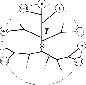
The idea behind our pruning comes from an existing polynomial-time algorithm for a special case of Steiner tree such that the input graph is planar and all the terminals are on a single face. In this case, we can improve the running time of the FPT algorithm toO(k3_n+k2_{nlogn)as follows}

(Erickson, Monma, and Veinott 1987). We number the ter-minals from0 tok−1 along the face they locate on (see Figure 1). LetT be a minimum Steiner tree for the

termi-2

https://github.com/wata-orz/steiner tree

𝒌−𝟏 𝟎 𝟏

𝑻

𝒔+𝟏 𝒔−𝟏

𝒕−𝟏

𝒖 𝒕+𝟏

𝒔 𝒕

Figure 1: All the terminalsA={0,1, . . . , k−1}are on the unbounded face. By splitting a Steiner treeT atu∈V(T), we obtain two Steiner trees for terminals{s, s+ 1, . . . , t} ∪ {u}and{t+ 1, t+ 2, . . . , s−1} ∪ {u}.

nals A. Because the graph is planar and all the terminals are on a single face, we can see that for any two terminals s, t ∈ A, the path betweensandtonT separatesthe ter-minals{s+ 1, . . . , t−1}from the others. Letu ∈ V(T) be a vertex on T. By splitting T at u, we can cut out a minimum Steiner tree for terminalsS∪ {u}for some sub-set S ⊆ A. By the above property, we can assume that S induces a consecutive interval of A; i.e., we can write S = {s, s+ 1, . . . , t−1, t} for some integers s, t ≥ 0 (whens > t, we use modulok). Therefore, in the dynamic programming, it is sufficient to compute a minimum Steiner tree for terminalsS∪ {u}only for every such consecutive intervalS ⊆A. As the number of such intervals isO(k2_),

we obtain the above running time.

We can apply this idea for general inputs as follows. Sup-pose that we have computed a minimum Steiner treeT for terminalsS∪ {u}for some subsetS ⊆ Aandu ∈ V by the dynamic programming. If the remaining terminalsA\S are separated byV(T)\ {u}, any minimum Steiner tree for (A\S)∪ {u} must contain some vertex in V(T)\ {u}. Therefore, we immediately know that the current minimum Steiner tree forS∪ {u}cannot be extended to a minimum Steiner tree forA, and thus we can discard it from the DP table. In contrast to the previous special case, unfortunately, this condition rarely happens for general inputs. Our key ob-servation is that, even ifV(T)\ {u}itself is not a separator, we can apply the pruning if there exists a separator satisfying some weaker condition. As in the previous special case, this pruning significantly reduces the number of subsetsS ⊆A we need to consider (especially, for sparse graphs admitting small separators) and thus leads to a significant speedup.

Preliminaries

Algorithm 1(Erickson, Monma, and Veinott 1987) 1: d(S, u)← ∞for∀S⊆Aand∀u∈V. 2: d({a}, a)←0for∀a∈A.

3: forS⊆Ain ascending order of|S|do 4: Initialize a priority queueQdonV. 5: whileQdis not emptydo

6: Popuwith the smallestd(S, u)value fromQd. 7: foruv∈Edo

8: d(S, v)←−−min d(S, u) +w(uv) 9: foralready processedS0⊆A\Sdo 10: foru∈V do

11: d(S∪S0, u)←−−min d(S, u) +d(S0, u) 12: returnd(A, a)for an arbitrarya∈A.

anS-separatorifS∩C 6= ∅orS is not connected in the graph G[V \C]; or in other words, every Steiner tree for Scontains some vertex inC. For a treeT and two vertices uandvonT, we defineb(T, u, v)as the maximum weight of a maximal degree-two path contained in the unique path betweenuandv inT3_{. Given a treeT and a vertexu, we}

can computeb(T, u, v)for allv ∈ V(T)in linear time by a simple DFS fromu. For a variablexand a valuey, we denote byx←−−min yan operation updatingx←min(x, y).

Classical Algorithm

We review a classicalO(3kn+ 2k(m+nlogn))-time DP algorithm (Erickson, Monma, and Veinott 1987) described in Algorithm 1. We first create a two-dimensional tabled :

2A_{×V →}

R≥0, which is initialized asd({a}, a) = 0for

every terminala∈Aandd(S, u) =∞for every otherS⊆

Aandu∈V. We store the minimum weight of a Steiner tree forS∪ {u}we have found so far ind(S, u). We compute the table by processing each subsetS ⊆ A one by one in ascending order of the size|S|. After processing a subsetS, we ensure thatd(S, u)is equal toopt(S∪ {u})for every u ∈ V. Finally, we can solve the problem by answering d(A, a)for an arbitrary terminala∈A.

We process each subsetS ⊆Aas follows. First, we up-date d(S, u) for every u by using Dijkstra’s algorithm as follows; while there are unprocessed vertices, we pop an unprocessed vertex u with the smallest d(S, u) value by using a priority queue; then for each edge uv ∈ E, we update d(S, v) ←−−min d(S, u) + w(uv) (we can obtain a Steiner tree forS∪ {v}by inserting the edgeuvto a Steiner tree forS∪ {u}). This takesO(m+nlogn)time by us-ing the Fibonacci heap. After this update, for each subset S0 ⊆ A\S that has been already processed, we update d(S ∪ S0, u) ←−−min d(S, u) + d(S0, u) (we can obtain a Steiner tree forS∪S0∪{u}by merging two Steiner trees for S∪ {u}andS0_{∪ {u}). This takesO(2}k−|S|_{n)time. Thus}

3

Suppose that the path between u = v0 and v = v` is

(v0, v1, . . . , v`), and among these vertices,{vi1, . . . , vip}have

de-gree at least three inT. Then(v0, . . . , vi1),(vi1, . . . , vi2),. . ., and

(vip, . . . , v`)are the set of maximal degree-two paths.

the total running time isP

S⊆A(m+nlogn+ 2

k−|S|_{n) =}

O(3k_{n+ 2}k_(m+nlogn)).

Separator-based Pruning

In order to speed up the DP algorithm, instead of computing d(S, u)for everyS ⊆ V andu∈ V, we compute a small portion of them while maintaining correctness of the algo-rithm. For a subsetS⊆V, we denote byvalid(S)the set of verticesv ∈ V such that(S, v)is contained in the tabled. Because we expect thatvalid(S) =∅for a large portion of subsetsS⊆A, instead of using the two-dimensional array, we use a binary search tree to efficiently maintain the table d. The key in each node is a setS ⊆Awithvalid(S)6=∅, and the value is a list of(u, d(S, u))foru∈valid(S).

For a subsetS ⊆Aand a vertexu∈V, a Steiner treeT forS∪ {u}is calledimportantif there exists a Steiner tree T0_{for(A\S)∪ {u}such thatT+T}0_{is a minimum Steiner}

tree forA. We can easily see that the optimal solution can be obtained by computing onlyd(S, u)such that the minimum Steiner tree forS∪ {u}is important; however, it is difficult to test the importance without knowing the optimal solution itself. In our algorithm, we use the following necessary con-dition of the importance.

Lemma 1. For a subset S ⊆ A and a vertex u ∈ V, a Steiner treeTforS∪ {u}is not important if there exists an

(A\S)-separatorCsuch that, for everyv∈C, there exists

Sv ⊆Ssatisfying the following inequality:

opt(Sv∪ {v}) + opt((S\Sv)∪ {u})< w(T). (1) Proof. Suppose that T is important. Then there exists a Steiner treeT0_{for(A\S)∪ {u}such thatT+T}0_{is a}

mini-mum Steiner tree forA. BecauseCis an(A\S)-separator, T0 must contain some vertexv ∈C. LetTv be a minimum Steiner tree forSv∪ {v}and letTube a minimum Steiner tree for(S\Sv)∪ {u}. ThenTv+Tu+T0is a Steiner tree forAsatisfyingw(Tv+Tu+T0)< w(T+T0), which is a contradiction.

In our algorithm, after processing a subsetS ⊆ A, we ensure the following for everyu ∈ V: (1) if the minimum Steiner tree forS∪ {u}is important,(S, u)is contained in the tabledandd(S, u)is equal toopt(S∪ {u})and (2) if it is not important,(S, u)is not contained indord(S, u)is at leastopt(S∪ {u}).

A special case of Lemma 1 is when Sv = S for every v ∈ C. In this case, the inequality (1) can be simplified to opt(S∪ {v})< w(T). We can exploit this special case as follows. For a valuex, we defineCx:={v|d(S, v)≤x}. Before running the for-loops at lines 9–11, we compute the minimum valuexsuch thatCxforms an(A\S)-separator. We then know thatopt(S∪ {v})≤d(S, v) ≤xholds for every v ∈ Cx. Therefore we can conclude that for every u∈V withd(S, u)> x, the corresponding Steiner tree for S∪ {u}is not important, and thus we can safely drop(S, u) from the table.

Lemma 2. For a subsetS ⊆ A and a vertex u ∈ V, a Steiner treeT forS∪ {u}is not important if there exists an

(A\S)-separatorCsuch that, for everyv∈C, at least one of the following two conditions is satisfied.

1. opt(S∪ {v})< w(T), or

2. there exists a vertexs∈V(T)such that the distance be-tweensandvis less thanb(T, u, s).

Proof. We prove the lemma by applying Lemma 1. Letvbe a vertex inC. Ifvsatisfies the first condition, the inequality (1) holds forSv =S. Ifvsatisfies the second condition, let P be a maximum-weight degree-two path contained in the path betweenuandsonT (so we havew(P) =b(T, u, s)). By deletingPfromT, we obtain a Steiner tree forS0∪ {s}

and a Steiner tree for(S\S0)∪ {u}for someS0⊆Swhose total weight isw(T)−w(P). Therefore, we haveopt(S0∪ {s})+opt((S\S0)∪{u})≤w(T)−w(P). Because we can construct a Steiner tree forS0∪{v}by inserting the shortest-path betweensandvto a Steiner tree forS0∪ {s}, we have opt(S0∪ {v})<opt(S0∪ {s}) +w(P). We now have

opt(S0∪ {v}) + opt((S\S0)∪ {u})

<opt(S0∪ {s}) +w(P) + opt((S\S0)∪ {u}) ≤(w(T)−w(P)) +w(P)

≤w(T).

Therefore, the inequality (1) holds forSv =S0.

We now describe the entire algorithm (see Algorithm 2). We iterate only over subsetsS ⊆ A such thatvalid(S)is non-empty. For a vertexu∈valid(S), we denote byTuthe corresponding Steiner tree forS∪ {u}of weightd(S, u).

Before running Dijkstra’s algorithm, we first apply the following update (lines 4–9). For each vertexu∈valid(S), we construct the corresponding Steiner treeTu. Because the Steiner tree Tu is also a Steiner tree for S ∪ {v} for ev-eryv ∈ V(Tu), we updated(S, v)

min

←−− d(S, u)for every v∈V(Tu). Note that, even ifTuis important forS∪ {u}, it may not be important forS∪ {v}, and therefore the tabled may not contain(S, v). We mark every suchvas ‘dummy’ so that we can identify the corresponding Steiner tree as unimportant. Although any Steiner tree obtained by extend-ing an unimportant Steiner tree is also unimportant, this up-date leads to smallerd(S, v)values for unimportant Steiner trees, and therefore it is helpful for pruning.

We then update the tabled by running Dijkstra’s algo-rithm (lines 10–16). This part is almost the same as the clas-sical algorithm without pruning. The only difference is that we propagate the ‘dummy’ mark.

Next, we compute a setNof vertices as follows (lines 17– 27). Letpbe a table initialized as follows: ifvis contained in everyTu, we setp(v)← −minu∈valid(S)b(Tu, u, v), and otherwise, we setp(v) ← 0. We updatepby running Di-jkstra’s algorithm with the initial distance pand then set N := {v | p(v) <0}. After this update,p(v)is the mini-mum of zero anddist(s, v)−minu∈valid(S)b(Tu, u, s)over all scontained in everyTu. Therefore, p(v) < 0 implies that, for everyu∈ valid(S), there existss ∈ V(Tu)such

Algorithm 2Separator-based Pruned DP Algorithm 1: d({a}, a)←0for∀a∈A.

2: forS⊆Awithvalid(S)6=∅in ascending orderdo 3: dummy(u)←falsefor∀u∈V.

4: foru∈valid(S)do

5: Tu←the Steiner tree forS∪ {u}. 6: forv∈V(Tu)do

7: ifd(S, v)> d(S, u)then 8: d(S, v)←d(S, u)

9: dummy(v)←true

10: Initialize a priority queueQdonV. 11: whileQdis not emptydo

12: Popuwith the smallestd(S, u)value fromQ. 13: foruv∈Edo

14: ifd(S, v)> d(S, u) +w(uv)then 15: d(S, v)←d(S, u) +w(uv)

16: dummy(v)←dummy(u)

17: forv∈V do

18: ifvis contained in everyTuthen 19: p(v)← −minu∈valid(S)b(Tu, u, v) 20: else

21: p(v)←0

22: Initialize a priority queueQponV. 23: whileQpis not emptydo

24: Popuwith the smallestp(u)value fromQp. 25: foruv∈Edo

26: p(v)←−−min p(u) +w(uv) 27: N ← {v|p(v)<0}.

28: x←minimumxs.t.(Cx∪N)is anA\S-separator. 29: foru∈V withd(S, u)> xordummy(u)do 30: Drop(S, u)fromd.

31: foralready processedS0⊆A\Sdo 32: foru∈valid(S)∩valid(S0)do

33: d(S∪S0, u)←−−min d(S, u) +d(S0, u) 34: returnd(A, a)for an arbitrarya∈A.

thatdist(s, v) < b(Tu, u, s). Thus, the second condition of Lemma 2 is satisfied for everyv∈N.

We now do pruning (lines 28–30). We compute a mini-mum valuexsuch thatCx∪N forms an(A\S)-separator (or zero ifN itself is an(A\S)-separator), whereCx :=

{v | d(S, v) ≤ x}. We can efficiently compute suchxas follows; starting from an empty set R, we insert a vertex v ∈ V \N to R one by one in non-increasing order of d(S, v); when all the vertices inA\Sget connected inG[R], we setx :=d(S, v)for the last inserted vertexv. Letube a vertex with d(S, u) > x. For each vertex v ∈ Cx, the first condition of Lemma 2 is satisfied, and for each vertex v∈N, the second condition of Lemma 2 is satisfied. There-fore, we can safely drop every(S, u)withd(S, u)> xfrom the tabledby applying Lemma 2. We can also drop(S, u) for everyu∈V with the ‘dummy’ mark because we know that the corresponding Steiner tree is unimportant.

Steiner tree forS0∪ {u}into a Steiner tree forS∪S0∪ {u}

(lines 31–33). This part is almost the same as the classical algorithm without pruning. The only difference is how to enumerate all suchS0. Because we only need to enumerate subsetsS0 ⊆A\Swithvalid(S)∩valid(S0)6=∅, we use a sophisticated data structure presented in the next section.

Further Speed-up Techniques

We present two techniques for further speeding up the pruned DP algorithm.

Data Structure

We propose a binary tree data structure to maintain a set of already processed subsets S0 ⊆ A withvalid(S0) 6= ∅so that, given a subsetS⊆A, we can efficiently enumerate all the subsetsS0 ⊆A\Swithvalid(S)∩valid(S0)6=∅. For a nodei, letLidenote the set of leaves of the subtree rooted ati. For two subsetsS, S0 ⊆A, we definep(S, S0)as the minimum integerpsuch thatS∩[p]andS0∩[p]differ.

Each leaftof the tree contains a setSt⊆A. Each internal nodeiof the tree contains an integerkiand two setsIi⊆A andUi ⊆V. Initially, the data structure consists of a single leaftwithSt=∅. We maintain the data structure so that the following holds for every internal nodei.

1. Ii=∩t∈LiSt. 2. Ui=∪t∈Livalid(St).

3. For allt∈Li,St∩[ki−1]is the same.

4. For the left childl,ki6∈Stfor allt∈Ll, and for the right childr,ki∈Stfor allt∈Lr.

We insert a subsetS ⊆ A into the data structure by re-cursively applying the following procedure starting from the root. If the current nodel is a leaf, we create a new inter-nal nodeiwithIi :=Sl∩S,Ui := valid(Sl)∪valid(S), andki :=p(Sl, S); create a new leafrwithSr :=S; and then replace l with the node i having two children l and r. If the current nodeiis an internal node andp(Ii, S) < ki, we create a new internal node j with Ij := Ii ∩S, Uj := Ui ∪valid(S), and kj := p(Ii, S); create a new leaf r withSr := S; and then replace i with the node j having two childreniandr. If the current nodeiis an in-ternal node andp(Ii, S)≥ki, we updateIi ←Ii∩Sand Ui ← Ui ∪valid(S); and then proceed to the left child if ki 6∈ Sor to the right child ifki ∈ S. The worst-case run-ning time of the insertion isO(kn).

We enumerate subsets S0 ⊆ A \ S with valid(S) ∩ valid(S0) 6= ∅ by recursively applying the following pro-cedure starting from the root. If the current nodetis a leaf, we check the condition forStand add it to the candidates. If the current nodeiis an internal node withIi∩S 6=∅or Ui∩valid(S) =∅, we immediately know thatLicontains no subsetsS0 ⊆A\Swithvalid(S0)∩valid(S)6=∅. There-fore, we do not process its children. If the current nodeiis an internal node withIi∩S = ∅andUi∩valid(S) 6= ∅, we recursively process the two children ofi. The worst-case running time of the enumeration isO(min(2k−|S|_,|L|)n),

whereLis the set of subsets inserted into the data structure.

Note that our data structure is completely useless for the un-pruned version becausevalid(S) =V holds for allS ⊆A.

Meet in the Middle

We use the following folklore lemma about the existence of a balanced separation of a tree (for the proof, see, e.g., (Fomin et al. 2018)) to show that we can obtain a minimum Steiner tree by merging three Steiner trees for small subsets. Lemma 3. Let T be a tree andµ : V(T) → R≥0 be a

non-negative vertex weight function. Then there exists a ver-texu∈ V(T)such thatµ(V(C))≤µ(V(T))/2for every connected componentCofT−u.

Corollary 1. LetTbe a minimum Steiner tree forA. When

|A| ≥ 3, there exists a vertex u ∈ V(T)and a partition

A =S1∪S2∪S3with1 ≤ |S1| ≤ |S2| ≤ |S3| ≤ |A|/2

such thatTis a union of Steiner trees forS1∪{u},S2∪{u},

andS3∪ {u}.

Proof. By applying Lemma 3 againstµ:V → {0,1}such thatµ(u) = 1 ⇐⇒ u∈A, we obtain a vertexu0 ∈V(T) such that each connected component ofT −u0 contains at most |A|/2terminals. Letube a vertex of degree at least three or contained in A that is nearest to u0 on T. Then, we obtain a partitionA = S1∪. . .∪Sd withd ≥ 3and

1 ≤ |Si| ≤ |A|/2 for each Si such that T is a union of Steiner trees forS1∪{u},. . ., andSd∪{u}. Whiled≥4, we pick two smallestSiandSj and then replace them with the unionSi∪Sj. Note that becaused≥4,|Si|+|Sj| ≤ |A|/2 holds. Finally, whendbecomes three, we obtain the desired partition.

Using this corollary, we can speed up the algorithm as follows. In the for-loop at line 2, we iterate only over subsets S ⊆Aof size at most|A|/2. In the for-loop at line 31, we iterate only over subsetsS0 ⊆A\Sof size at most|A| − 2|S|. Finally, we return the minimum ofd(S, u)+d(A\S, u) over all the processedSandu∈valid(S).

Lemma 4. The above speedup is correct.

Proof. LetS1, S2, S3be the subsets in Corollary 1. Because

the size of each subset is at most|A|/2, the algorithm cor-rectly computes a minimum Steiner tree forSi∪ {u}for ev-eryi∈[3]. Becauseopt(S1∪S2∪ {u}) = opt(S1∪ {u}) +

opt(S2∪ {u})and we have|S1| ≤ |A| −2|S2|, it also

cor-rectly computes a minimum Steiner tree forS1∪S2∪ {u}.

Therefore,d(S3, u)+d(A\S3, u) =d(S3, u)+d(S1∪S2, u)

gives the minimum Steiner tree.

Experimental Evaluation

We conducted experiments on a Linux server with Intel Xeon E5-2670 (2.6 GHz) which produced a score of 399 for the DIMACS benchmark. For each test, we use a sin-gle thread and limit the maximum run time by 30 minutes and the maximum memory by 6GB. In the experiments, we use the following benchmark datasets used in the DIMACS challenge and the PACE challenge.

Random (B, C, D, E, MC, I, P4Z, P6Z): random graphs. Artificial (SP, PUC): artificial instances.

Euclidian (X, P4E, P6E): Euclidian graphs. CrossGrid (1R, 2R): 2D/3D cross-grid graphs.

VLSI (ALUE, ALUT, DIW, DMXA, GAP, MSM, TAQ, LIN): grid graphs with holes coming from VLSI appli-cations.

Rectilinear (ESFST, TSPFST): rectilinear graphs with L1 distances preprocessed with GeoSteiner (Warme, Winter, and Zachariasen 2000).

Group (WRP): instances obtained by a reduction from the group Steiner tree problem coming from industrial wire routing problems (Zachariasen and Rohe 2003). Vienna Real-world instances from telecommunication

net-works (Leitner et al. 2014).

Copenhagen Obstacle-avoiding rectilinear Steiner tree in-stances preprocessed with ObSteiner (Huang and Young 2013).

PACE Public instances of the two exact tracks of the PACE challenge, each of which consists of 100 instances from SteinLib and Vienna.

Impact of Pruning

We first evaluate the impact of the pruning by comparing the performance with the unpruned version EMV ((Erickson, Monma, and Veinott 1987)) using the PACE dataset. Note that EMV is not a state-of-the-art method but a baseline al-gorithm. Because the performance depends on the type of instances, we will give a detailed comparison with two mod-ern solvers later in this section. For evaluating the effect of the two speed-up techniques, we implemented three variants of the pruned DP algorithm: PRUNED(DS,MM) uses both of the two speed-up techniques, PRUNED(DS) uses the data structure but does not use the meet-in-the-middle technique, and PRUNED(∅) uses neither techniques. PRUNED(∅) keeps the processed subsets in a list and enumerates all the subsets S0⊆A\Swithvalid(S)∩valid(S0)6=∅by naively testing all the subsets in the list. All the solvers were implemented using the Rust programming language.

The cactus plot in Figure 2 shows the running time of each solver. We can see that PRUNED(∅) is already quite faster than EMV. The data structure improves the performance against difficult instances, and the meet-in-the-middle leads to a uniform speedup. In the subsequent experiments, we will use PRUNEDto refer to the solver PRUNED(DS,MM).

Figure 3 illustrates the effect of the number of terminals k. A point at coordinates(k, t)means that an instance with k terminals was solved int seconds. We can see that the running time of EMV exponentially depends onk but the running time of PRUNEDdoes not. While there are unsolved instances with only25terminals, there also exist solved in-stances with more than a thousand terminals. This is not so surprising when recalling that the idea of the proposed prun-ing came from the polynomial-time algorithm for special planar instances for which the number of subsets of termi-nals we need to consider is notexp(k)butO(k2_{). Hence the}

effectiveness of the pruning strongly depends on structures

0 25 50 75 100 125 150 175 200

the number of instances 10 3

10 2 10 1 100 101 102 10TLE3

running time [sec]

EMV Pruned(DS,MM) Pruned(DS) Pruned( )

Figure 2: A cactus plot showing the running times of EMV and the three variants of PRUNED.

10

₁₀

₁₀

₁₀

the number of terminals k

10

10

10

running time t [sec]

EMV

Pruned

Figure 3: Effect of the number of terminalsk

of graphs (e.g., we can expect that the pruning will be effec-tive for sparse graphs admitting many small separators, but it will not be effective for dense or random graphs).

Comparison with the

A

Search

We compare the performance of PRUNEDwith an existing solver HSV (Hougardy, Silvanus, and Vygen 2017) using the experimental results reported in their paper. Their ex-periments were conducted on a computer with Intel Xeon W5590 (3.33 GHz) which produced a score of 391 for the DIMACS benchmark and their solver was implemented us-ing C++ language. HSV combines the EMV algorithm and the A∗ search as follows: instead of filling the DP table d(S, u)from small|S|to large|S|, it computes some lower boundµ(A\S, u)ofopt(A\S, u)and processes the one with the smallestd(S, u) +µ(A\S, u)value using a prior-ity queue. It also uses a pruning based on the lower bound µ. Note that it seems difficult to combine theA∗search with our separator-based pruning because, in order to efficiently obtain the separator used in our pruning, we need to com-pute the values ofd(S, u)for allu ∈ V at once. Because HSV did not use any preprocessing, we run PRUNED with-out preprocessing for a fair comparison.

num-Table 1: Comparison of HSV and PRUNED

HSV PRUNED

Dataset # solved better solved better

Random 418 262 0 281 35

Artificial 21 11 0 11 0

Euclidian 26 26 0 26 0

CrossGrid 45 33 0 42 14

VLSI 128 128 1 128 0

Rectilinear 93 93 0 93 4

Group 89 16 0 87 82

Vienna 6 3 0 6 3

Copenhagen 10 10 0 10 0

103 ₁₀2 ₁₀1 ₁₀0 ₁₀1 ₁₀2 ₁₀3_TLE

running time of HSV [sec] 10 3

10 2 10 1 100 101 102 103 TLE

running time of Pruned [sec]

Random Artificial Euclidian CrossGrid VLSI Rectilinear Group Vienna Copenhagen

Figure 4: Running time comparison of HSV and PRUNED

ber of instances for which the solver performed significantly better than the other; we say that the performance of a solver s1is significantly better than a solvers2for an instanceiif

either (1)s1solvedibuts2did not or (2) both of them solved

ibut the run time of s2 is greater than the run time of s1

times ten plus one second. Figure 4 illustrates the running time comparison against each instance. Each point corre-sponds to a single instance and its coordinates(x, y)means that HSV solved the instance in xseconds and PRUNED

solved the instance inyseconds.

We can see that PRUNEDoutperforms HSV for datasets Random, CrossGrid, Group, and Vienna. For Random, the pruning is not so effective butA∗ search is not even more effective. For the other three datasets, the pruning works ef-fectively because they are near-planar.

Comparison with the Branch-and-Cut Method

We compare the performance of PRUNED with an open-source branch-and-cut solver SCIP-JACK (Gamrath et al. 2017). We use the latest version of SCIP-JACKwhich has been submitted to the PACE challenge and won the 3rd in the track 1 and the 1st in the track 2. It internally uses an MIP

Table 2: Comparison of SCIP-JACKand PRUNED

SCIP-JACK PRUNED

Dataset # k/n solved better solved better

Random 133 .256 96 91 16 0

Artificial 53 .239 8 4 6 6

VLSI 40 .046 20 0 32 27

Rectilinear 143 .425 138 41 113 1

Group 85 .086 65 4 79 58

Vienna 210 .145 129 97 42 7

Copenhagen 12 .140 8 2 7 3

103 ₁₀2 ₁₀ 1 ₁₀0 ₁₀1 ₁₀2 ₁₀3_TLE

running time of SCIP-Jack [sec] 103

102 101 100 101 102 103 TLE

running time of Pruned [sec]

Figure 5: Running time comparison of SCIP-JACK and PRUNED. The legend is the same as in Figure 4.

solver SCIP (Gleixner et al. 2018) version 5.0.1 and an LP solver SoPlex (Gleixner, Steffy, and Wolter 2012; 2015) ver-sion 3.1.1. In addition to the branch-and-cut method, SCIP-JACK uses a variety of preprocessing techniques to reduce the graph size (Rehfeldt 2015). In the following compari-son, PRUNED also uses the same preprocessing as SCIP-JACKand the run time for the preprocessing is excluded for both solvers so that the difference between the pruned DP algorithm and the branch-and-cut method becomes clear.

Table 2 and Figure 5 show the comparison of the perfor-mance of SCIP-JACKand PRUNEDagainst datasets SteLib, Vienna, and Copenhagen. We omit all the too-easy in-stances for which the preprocessing alone solved the prob-lem. The column ‘#’ shows the number of the remaining instances in each dataset, and the column ‘k/n’ shows the average ofk/nin the dataset. Because the theoretical worst-case running time of SCIP-JACK and PRUNED exponen-tially depends onnandk, respectively, we can expect that a dataset with a smallerk/nvalue is more advantageous to PRUNED. Note that the table does not contain Euclidian and CrossGrid because the preprocessing solved all the instances in these datasets.

Ran-dom is bad because ranRan-dom graphs admit no small separa-tors. PRUNED outperforms SCIP-JACK against VLSI and Group both coming from industrial applications. This is due to the following two reasons: (1) the number of terminals is relatively small for these applications (the number of termi-nals of an instance obtained by the reduction from the Group Steiner tree is the number of groups) and (2) because the graphs are grid with holes, they admit many small separa-tors. On the other hand, SCIP-JACK outperforms PRUNED

against geometric datasets Rectilinear and Vienna.

Acknowledgments

Yoichi Iwata is supported by JSPS KAKENHI Grant Num-ber JP17K12643.

References

Althaus, E., and Blumenstock, M. 2014. Algorithms for the maximum weight connected subgraph and prize-collecting steiner tree problems. 11th DIMACS Implementation Chal-lenge Workshop (Technical Report).

Bodlaender, H. L.; Cygan, M.; Kratsch, S.; and Nederlof, J. 2015. Deterministic single exponential time algorithms for connectivity problems parameterized by treewidth. Inf. Comput.243:86–111.

Cygan, M.; Dell, H.; Lokshtanov, D.; Marx, D.; Nederlof, J.; Okamoto, Y.; Paturi, R.; Saurabh, S.; and Wahlstr¨om, M. 2016. On problems as hard as CNF-SAT. ACM Trans. Al-gorithms12(3):41:1–41:24.

Daneshmand, S. V. 2004. Algorithmic approaches to the Steiner problem in networks. Ph.D. Dissertation, Universit¨at Mannheim.

Ding, B.; Yu, J. X.; Wang, S.; Qin, L.; Zhang, X.; and Lin, X. 2007. Finding top-k min-cost connected trees in databases. InICDE, 836–845.

Dreyfus, S. E., and Wagner, R. A. 1971. The steiner problem in graphs.Networks1(3):195–207.

Duin, C. 2000. Preprocessing the steiner problem in graphs. InAdvances in Steiner Trees. Springer US. 175–233. Erickson, R. E.; Monma, C. L.; and Veinott, A. F. 1987. Send-and-split method for minimum-concave-cost network flows.Math. Oper. Res.12(4):634–664.

Fafianie, S.; Bodlaender, H. L.; and Nederlof, J. 2015. Speeding up dynamic programming with representative sets: An experimental evaluation of algorithms for steiner tree on tree decompositions.Algorithmica71(3):636–660.

Fischetti, M.; Leitner, M.; Ljubic, I.; Luipersbeck, M.; Monaci, M.; Resch, M.; Salvagnin, D.; and Sinnl, M. 2017. Thinning out steiner trees: a node-based model for uniform edge costs.Math. Program. Comput.9(2):203–229. Fomin, F. V.; Lokshtanov, D.; Saurabh, S.; Pilipczuk, M.; and Wrochna, M. 2018. Fully polynomial-time parameter-ized computations for graphs and matrices of low treewidth.

ACM Trans. Algorithms14(3):34:1–34:45.

Fuchs, B.; Kern, W.; M¨olle, D.; Richter, S.; Rossmanith, P.; and Wang, X. 2007. Dynamic programming for minimum steiner trees.Theory Comput. Syst.41(3):493–500.

Gamrath, G.; Koch, T.; Maher, S. J.; Rehfeldt, D.; and Shi-nano, Y. 2017. SCIP-Jack - a solver for STP and variants with parallelization extensions. Math. Program. Comput.

9(2):231–296.

Gleixner, A.; Bastubbe, M.; Eifler, L.; Gally, T.; Gam-rath, G.; Gottwald, R. L.; Hendel, G.; Hojny, C.; Koch, T.; L¨ubbecke, M. E.; Maher, S. J.; Miltenberger, M.; M¨uller, B.; Pfetsch, M. E.; Puchert, C.; Rehfeldt, D.; Schl¨osser, F.; Schubert, C.; Serrano, F.; Shinano, Y.; Viernickel, J. M.; Walter, M.; Wegscheider, F.; Witt, J. T.; and Witzig, J. 2018. The SCIP Optimization Suite 6.0. ZIB-Report 18-26, Zuse Institute Berlin.

Gleixner, A. M.; Steffy, D. E.; and Wolter, K. 2012. Im-proving the accuracy of linear programming solvers with it-erative refinement. InISSAC, 187–194.

Gleixner, A. M.; Steffy, D. E.; and Wolter, K. 2015. Iterative refinement for linear programming. Technical Report 15-15, ZIB, Takustr. 7, 14195 Berlin.

Held, S.; Korte, B.; Rautenbach, D.; and Vygen, J. 2011. Combinatorial optimization in VLSI design. In Combina-torial Optimization - Methods and Applications. IOS Press. 33–96.

Hougardy, S.; Silvanus, J.; and Vygen, J. 2017. Dijkstra meets steiner: a fast exact goal-oriented steiner tree algo-rithm. Math. Program. Comput.9(2):135–202.

Huang, T., and Young, E. F. Y. 2013. Obsteiner: An ex-act algorithm for the construction of rectilinear steiner min-imum trees in the presence of complex rectilinear obstacles.

IEEE Trans. on CAD of Integrated Circuits and Systems

32(6):882–893.

Koch, T.; Martin, A.; and Voß, S. 2000. SteinLib: An up-dated library on steiner tree problems in graphs. Technical Report ZIB-Report 00-37, Konrad-Zuse-Zentrum f¨ur Infor-mationstechnik Berlin, Takustr. 7, Berlin.

Lappas, T.; Liu, K.; and Terzi, E. 2009. Finding a team of experts in social networks. InKDD, 467–476.

Leitner, M.; Ljubic, I.; Luipersbeck, M.; Prossegger, M.; and Resch, M. 2014. New real-world instances for the steiner tree problem in graphs.Technical Report, ISOR, Uni Wien. Marx, D.; Pilipczuk, M.; and Pilipczuk, M. 2017. On subex-ponential parameterized algorithms for steiner tree and di-rected subset TSP on planar graphs. CoRRabs/1707.02190. Polzin, T. 2004. Algorithms for the Steiner problem in net-works. Ph.D. Dissertation, Saarland University.

Rehfeldt, D. 2015. A generic approach to solving the steiner tree problem and variants. Master’s thesis, Technische Uni-versit¨at Berlin.

Warme, D.; Winter, P.; and Zachariasen, M. 2000. Exact algorithms for plane Steiner tree problems: A computational study. In Du, D.-Z.; Smith, J.; and Rubinstein, J., eds., Ad-vances in Steiner Trees. Kluwer. 81–116.