Algorithms for Estimating Trends in Global Temperature Volatility

(1)

The Thirty-Third AAAI Conference on Artificial Intelligence (AAAI-19)

Algorithms for Estimating Trends

in Global Temperature Volatility

Arash Khodadadi, Daniel J. McDonald

Department of Statistics

Indiana University Bloomington, IN 47408 {arakhoda,dajmcdon}@indiana.edu

Abstract

Trends in terrestrial temperature variability are perhaps more relevant for species viability than trends in mean temperature. In this paper, we develop methodology for estimating such trends using multi-resolution climate data from polar orbiting weather satellites. We derive two novel algorithms for com-putation that are tailored for dense, gridded observations over both space and time. We evaluate our methods with a simula-tion that mimics these data’s features and on a large, publicly available, global temperature dataset with the eventual goal of tracking trends in cloud reflectance temperature variability.

1 Introduction

The amount of sunlight reflected from clouds is among the largest sources of uncertainty in climate prediction (Boucher et al. 2013). But climate models fail to reproduce global cloud statistics, and understanding the reasons for this failure is a grand challenge of the World Climate Research Pro-gramme (Bony et al. 2015). While numerous studies have examined the overall impacts of clouds on climate variabil-ity (Myers, Mechoso, and DeFlorio 2018; Grise et al. 2013; Bender, Ramanathan, and Tselioudis 2012), such investiga-tions have been hampered by the lack of a suitable dataset. Ideal data would have global coverage at high spatial res-olution, a long enough record to recover temporal trends, and be multispectral (Wielicki et al. 2013). To address this gap, current work (Staten et al. 2016; Schreier et al. 2010; Kahn et al. 2007) seeks to create a spectrally-detailed dataset by combining radiance data from Advanced Very High Resolution Radiometer imagers with readings from High-resolution Infrared Radiation Sounders, instruments onboard legacy weather satellites. In anticipation of this new dataset, our work develops novel methodology for examining the trends in variability of climate data across space and time.

1.1 Variability Rather Than Average

Trends in terrestrial temperature variability are perhaps more relevant for species viability than trends in mean temper-ature (Huntingford et al. 2013), because an increase in temperature variability will increase the probability of ex-treme hot or cold outliers (Vasseur et al. 2014). Recent

climate literature suggests that it is more difficult for so-ciety to adapt to these extremes than to the gradual increase in the mean temperature (Hansen, Sato, and Ruedy 2012; Huntingford et al. 2013). Furthermore, the willingness of pop-ular media to emphasize the prevalence extreme cold events coupled with a fundamental misunderstanding of the rela-tionship between climate (the global distribution of weather over the long run) and weather (observed short-term, local-ized behavior) leads to public misunderstanding of climate change. In fact, a point of active debate is the extent to which the observed increased frequency of extreme cold events in the northern hemisphere can be attributed to increases in temperature variance rather than to changes in mean climate (Screen 2014; Fischer, Beyerle, and Knutti 2013; Trenberth et al. 2014).

Nevertheless, research examining trends in the volatility of spatio-temporal climate data is scarce. Hansen, Sato, and Ruedy (2012) studied the change in the standard deviation (SD) of the surface temperature in the NASA Goddard Insti-tute for Space Studies gridded temperature dataset by exam-ining the empirical SD at each spatial location relative to that location’s SD over a base period and showed that these esti-mates are increasing. Huntingford et al. (2013) took a similar approach in analyzing the ERA-40 data set. They argued that, while there is an increase in the SDs from 1958-1970 to 1991-2001, it is much smaller than found by Hansen, Sato, and Ruedy (2012). Huntingford et al. (2013) also computed the time-evolving global SD from the detrended time-series at each position and argued that the global SD has been stable. These and other related work (e.g., Rhines and Huybers 2013) have several shortcomings which our work seeks to remedy. First, no statistical analysis has been performed to examine if the changes in the SD are statistically significant. Second, the methodologies for computing the SDs are highly sensitive to the choice of base period. Third, and most impor-tantly, temporal and spatial correlations between observations are completely ignored.

(2)

strongly by increases in variance than by increases in mean. Finally, even if the global mean temperature is constant, there may still be climate change. In fact, atmospheric physics suggests that, across space, average temperatures should not change (extreme cold in one location is offset by heat in an-other). But if swings across space are becoming more rapid, then, even with no change in mean global temperature over time, increasing variance can lead to increases in the preva-lence of extreme events.

1.2 Main Contributions

The main contribution of this work is to develop a new methodology for detecting the trend in the volatility of spatio-temporal data. In this methodology, the variance at each position and time are estimated by minimizing the penalized negative loglikelihood. Following methods for mean estima-tion (Tibshirani 2014), we penalize the differences between the estimated variances which are temporally and spatially “close”, resulting in a generalized LASSO problem. How-ever, in our application, the dimension of this optimization problem is massive, so the standard solvers are inadequate.

We develop two algorithms which are computationally feasible on extremely large data. In the first method, we adopt an optimization technique called alternating direction method of multipliers (ADMM, Boyd et al. 2011), to divide the total problem into several sub-problems of much lower dimension and show how the total problem can be solved by iteratively solving these sub-problems. The second method, called linearized ADMM (Parikh and Boyd 2014), solves the main problem by iteratively solving a linearized version. We will compare the benefits of each method.

Our main contributions are as follows:

1. We propose a method for nonparametric variance estima-tion for a spatio-temporal process and discuss the rela-tionship between our methods and those existing in the machine learning literature (Section 2).

2. We derive two alternating direction method of multiplier algorithms to fit our estimator when applied to very large data (Section 3). We give situations under which each algorithm is most likely to be useful. Open-source Python code is available.1

3. Because the construction of satellite-based datasets is on-going and currently proprietary, we illustrate our methods on a large, publicly available, global temperature dataset. The goal is to demonstrate the feasibility of these meth-ods for tracking world-wide trends in variance in standard atmospheric data and a simulation constructed to mimic these data’s features (Section 4).

While the motivation for our methodology is its application to large, gridded climate data, we note that our algorithms are easily generalizable to spatio-temporal data under con-vex loss, e.g. exponential family likelihood. Furthermore the spatial structure can be broadly construed to include general graph dependencies. Our current application uses Gamma likelihood which lends itself well to modeling trends in pollu-tant emissions or in astronomical phenomena like microwave

1

github.com/dajmcdon/VolatilityTrend

background radiation. Volatility estimation in oil and natu-ral gas markets or with financial data is another possibility. Our methods can also be applied to resting-state fMRI data (though the penalty structure changes).

2 Smooth Spatio-temporal Variance

Estimation

Kim et al. (2009) proposed`1-trend filtering as a method for estimating a smooth, time-varying trend. It is formulated as the optimization problem

min

β

1 2

T

X

t=1

(yt−βt)2+λ T−1

X

t=2

|βt−1−2βt+βt+1|

or equivalently:

min

β

1

2ky−βk

2

2+λkDtβk1 (1) wherey ={yt}Tt=1 is an observed time-series,β ∈RT is the smooth trend,Dtis a(T −2)×T matrix, andλis a

tuning parameter which balances fidelity to the data (small errors in the first term) with a desire for smoothness. Kim et al. (2009) proposed a specialized primal-dual interior point (PDIP) algorithm for solving (1). From a statistical perspective, (1) can be viewed as a constrained maximum likelihood problem with independent observations from a normal distribution with common variance,yt∼N(βt, σ2),

subject to a piecewise linear constraint onβ. Alternatively, so-lutions to (1) are maximum a posteriori Bayesian estimators based on Gaussian likelihood with a special Laplace prior distribution onβ. Note that the structure of the estimator is determined by the penalty functionλkDtβk₁rather than any

parametric trend assumptions—autoregressive, moving aver-age, sinusoidal seasonal component, etc. The resulting trend is therefore essentially nonparametric in the same way that splines are nonparametric. In fact, using squared`2-norm as the penalty instead of`1results exactly in regression splines.

2.1 Modifications for Variance

Inspired by the`1-trend filtering algorithm, we propose a non-parametric model for estimating the variance of a time-series. To this end, we assume that at each time stept, there is a parameterhtsuch that the observationsytare independent

normal variables with zero mean and varianceexp(ht). The

negative log-likelihood of the observed data in this model is l(y | h) ∝ −P

tht−yt2e−ht. Crucially, we assume

that the parametershtvary smoothly and estimate them by

minimizing the penalized, negative log-likelihood:

min

h −l(y|h) +λkDthk1 (2)

whereDthas the same structure as above.

(3)

2.2 Adding Spatial Constraints

The method in the previous section can be used to estimate the variance of a single time-series. Here we extend this method to the case of spatio-temporal data.

At a specific timet, the data are measured on a grid of points with nr rows and nc columns for a total of S =

nr×nc spatial locations. Letyijt denote the value of the

observation at timeton theith row andjth column of the grid, andhijtdenote the corresponding parameter. We seek

to impose both temporal and spatial smoothness constraints on the parameters. Specifically, we seek a solution for h

which is piecewise linear in time and piecewise constant in space (although higher-order smoothness can be imposed with minimal alterations to the methodology). We achieve this goal by solving the following optimization problem:

min h

X

i,j,t

hijt+y2_ijte−hijt

+λtX

i,j

T−1

X

t=2

hij(t−1)−2hijt+hij(t+1)

(3)

+λsX

t,j

nr−1

X

i=1

hijt−h(i+1)jt

+λs

X

t,i

nc−1

X

j=1

hijt−hi(j+1)t

The first term in the objective is proportional to the neg-ative log-likelihood, the second is the temporal penalty for the time-series at each location(i, j), while the third and fourth, penalize the difference between the estimated vari-ance of two vertically and horizontally adjacent points, re-spectively. The spatial component of this penalty is a spe-cial case of trend filtering on graphs (Wang et al. 2016) which penalizes the difference between the estimated val-ues of the signal on the connected nodes (though the like-lihood is different). As before, we can write (3) in ma-trix form wherehis a vector of length T S and Dt is

re-placed byD ∈ R(Nt+Ns)×(T·S) _{(see Appendix C), where}

Nt=S·(T−2)andNs=T·(2nrnc−nr)are the number

of temporal and spatial constraints, respectively. Then, as we have two different tuning parameters for the temporal and spatial components, we writeΛ = λt1>Nt, λs1

>

Ns

>

leading to:2

min

h −l(y|h) + Λ

>_|_Dh_|_. ₍₄₎

2.3 Related Work

Variance estimation for financial time series has a lengthy history, focused especially on parametric models like the generalized autoregressive conditional heteroskedasticity (GARCH) process (Engle 2002) and stochastic volatility mod-els (Harvey, Ruiz, and Shephard 1994). These modmod-els (and related AR processes) are specifically for parametric mod-elling of short “bursts” of high volatility, behavior typical of financial instruments. Parametric models for spatial data go back at least to (Besag 1974) who proposed a conditional probability model on the lattice for examining plant ecology. More recently, nonparametric models for both spatial and temporal data have focused on using`1-regularization for

2

Throughout the paper, we use|x|for both scalars and vectors. For vectors we use this to denote a vector obtained by taking the absolute value of each entry ofx.

trend estimation. Kim et al. (2009) proposed`1-trend filter-ing for univariate time series, which forms the basis of our methods. These methods have been generalized to higher order temporal smoothness (Tibshirani 2014), graph de-pendencies (Wang et al. 2016), and, most recently, small, time-varying graphs (Hallac et al. 2017).

Our methodology is similar in flavor to (Hallac et al. 2017) or related work in (Gibberd and Nelson 2017; Monti et al. 2014), but with several fundamental differences. These pa-pers aim to discover the time-varying structure of a network. To achieve this goal, they use Gaussian likelihood with un-known precision matrix and introduce penalty terms which (1) encourage sparsity among the off-diagonal elements and (2) discourage changes in the estimated inverse covariance matrix from one time-step to the next. Our goal in the present work is to detect the temporal trend in the variance of each point in the network, but the network is known (correspond-ing to the grid over the earth) and fixed in time. To apply these methods in our context (e.g., Hallac et al. 2017, Eq. 2), we would enforce complete sparsity on the off-diagonal ele-ments (since they are not estimated) and add a new penalty to enforce spatial behavior across the diagonal elements. Thus, (4) is not simply a special case of these existing methods. Finally, these papers examine networks with hundreds of nodes and dozens to hundreds of time points. As discussed next, our data are significantly larger than these networks and attempting to estimate a full covariance would be prohibitive, were it necessary.

3 Optimization Methods

For a spatial grid of sizeSandTtime steps,Din Equation (4) will have3T S−2S−T nrrows andT Scolumns. For a

1◦×1◦grid over the entire northern hemisphere and daily data over 10 years, we haveS = 90×360≈32,000spatial locations andT = 3650time points, soDhas approximately

108columns and108rows. In principal, we could solve (4) using PDIP as before, however, each iteration requires solv-ing a linear system of equations which depends onD>D. Therefore, applying the PDIP directly is infeasible.3

In the next section, we develop two algorithms for solving this problem efficiently. The first casts the problem as a so-called consensus optimization problem (Boyd et al. 2011) which solves smaller sub-problems using PDIP and then recombines the results. The second uses proximal methods to avoid matrix inversions. Either may be more appropriate depending on the particular computing infrastructure.

3.1 Consensus Optimization

Consider an optimization problem of the formminhf(h),

where h ∈ Rn is the global variable and f(h) : Rn → R∪ {+∞}is convex. Consensus optimization breaks this

problem into several smaller sub-problems that can be solved independently in each iteration.

3

(4)

Figure 1: The cube represents the global variablehin space and time. The sub-cubes specified by the white lines arexi.

Assume it is possible to define a set of local variablesxi∈

Rni _{such that}_f₍_h_{) =}P

ifi(xi), where eachxiis a subset

of the global variableh. More specifically, each entry of the local variables corresponds to an entry of the global variable. Therefore we can define a mappingG(i, j)from the local variable indices into the global variable indices:k=G(i, j)

means that thejthentry ofxiishk(or(xi)j =hk). For ease

of notation, define˜hi ∈Rni _as_(˜_h

i)j =hG(i,j). Then, the

original optimization problem is equivalent to:

min {x1,...,xN}

N

X

i=1

fi(xi) s.t. ˜hi=xi. (5)

It is important to note that each entry of the global vari-able may correspond to several entries of the local varivari-ables and so the constraintsh˜i =xienforce consensus between

the local variables corresponding to the same global vari-able. The augmented Lagrangian corresponding to (5) is

Lρ(x, h, y) =Pi fi(xi)+u>i (xi−˜hi)+(ρ/2)kxi−˜hik22

. Now, we can apply ADMM toLρ. This results in solving

Nindependent optimization problems followed by a step to achieve consensus among the solutions in each iteration. To solve the optimization problem (4) using this method, we need to address two questions: first, how to choose the local variablesxi, and second, how to the update them.

In Figure 1, the global variablehis represented as a cube. We decomposehinto sub-cubes as shown by white lines. Each global variable inside the sub-cubes corresponds to only one local variable. The global variables on the border (white lines), however, correspond to more than one local variable. With this definition ofxi, the objective (4) decomposes as

P

ifi(xi)wherefi(xi) =−l(yi | xi) + Λ>(i)|D(i)xi|, and

Λ(i)andD(i)contain the temporal and spatial penalties corre-sponding toxionly in one sub-cube along with its boundary.

Thus, we now need to use PDIP to solveNproblems each of sizeni, which is feasible for small enoughni. Algorithm 1

gives the general version of this procedure. A more detailed discussion of this is in Appendix B of the Supplement where we show how to compute the dual and the derivatives of the augmented Lagrangian.

Because consensus ADMM breaks the large optimization into sub-problems that can be solved independently, it is

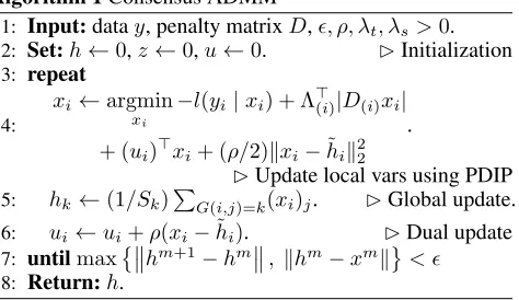
Algorithm 1Consensus ADMM

1: Input:datay, penalty matrixD,, ρ, λt, λs>0.

2: Set:h←0,z←0,u←0. _BInitialization 3: repeat

4:

xi←argmin xi

−l(yi|xi) + Λ(>i)|D(i)xi|

+ (ui)>xi+ (ρ/2)kxi−h˜ik22 .

BUpdate local vars using PDIP 5: hk ←(1/Sk)PG(i,j)=k(xi)j. BGlobal update.

6: ui←ui+ρ(xi−h˜i). BDual update

7: untilmax

hm+1₋_hm

, khm−xmk <

8: Return:h.

amenable to a split-gather parallelization strategy via, e.g., the MapReduce framework. In each iteration, the computation time will be equal to the time to solve each sub-problem plus the time to communicate the solutions to the master processor and perform the consensus step. Since each sub-problem is small, with parallelization, the computation time in each iteration will be small. In addition, our experiments with several values ofλtandλsshowed that the algorithm

converges in a few hundred iterations. This algorithm is most useful if we can parallelize the computation over several machines with low communication cost between machines. In the next section, we describe another algorithm which makes the computation feasible on a single machine.

3.2 Linearized ADMM

Consider the generic optimization problem minxf(x) +

g(Dx)wherex ∈ _Rn _and_D _∈

Rm×n. Each iteration of

the linearized ADMM algorithm (Parikh and Boyd 2014) for solving this problem has the form

x←prox

µf

x−(µ/ρ)D>(Dx−z+u)

z←prox

ρg

(Dx+u)

u←u+Dx−z

where the algorithm parametersµandρsatisfy0 < µ < ρ/kDk2₂,z, u ∈ Rmand the proximal operator is defined

asproxαϕ(u) = minx α·ϕ(x) +1₂kx−uk

2

2. Proximal algorithms are feasible when these proximal operators can be evaluated efficiently which, as we show next, is the case.

Lemma 1. Letf(x) =P

kxk+y

2

ke−xkandg(x) =kxk1. Then,

prox

µf

(u)

k =W

_y2

k

µ exp

₁₋_µu

k

µ

+1−µuk

µ ,

prox

ρg

(u) =Sρλ(u)

whereW(·)is the Lambert W function (Corless et al. 1996),

(5)

Algorithm 2Linearized ADMM

1: Input:datay, penalty matrixD,, ρ, λt, λs>0.

2: Set:h←0,z←0,u←0. _BInitialization 3: repeat

4: hk ← W

y2_k µ exp

1−µuk

µ

+ 1−µuk

µ for allk =

1, . . . T S. _BPrimal update

5: z←Sρλ(u). BElementwise soft thresholding

6: u←u−z. _BDual update

7: untilmax{kDh−zk, zm+1₋_zm }<

8: Return:z.

method for solving the same problem. In this case, both the primal update and the soft thresholding step are performed elementwise at each point of the spatio-temporal grid. It can therefore be extremely fast to perform these steps. However, because there are now many more dual variables, this algo-rithm will require more outer iterations to achieve consensus. It therefore is highly problem and architecture dependent whether Algorithm 1 or Algorithm 2 will be more useful in any particular context. In our experience, Algorithm 1 requires an order of magnitude fewer iterations, but each iteration is much slower unless carefully parallelized.

4 Empirical Evaluation

In this section, we examine both simulated and real spatio-temporal climate data. All the computations were performed on a Linux machine with four 3.20GHz Intel i5-3470 cores.

4.1 Simulations

Before examining real data, we apply our model to some synthetic data. This example was constructed to mimic the types of spatial and temporal phenomena observable in typ-ical climate data. We generate a complete spatio-temporal field wherein observations at all time steps and all locations are independent Gaussian random variables with zero mean. However, the variance of these random variables follows a smoothly varying function in time and space given by the following parametric model:

σ2(t, r, c) =

K

X

k=1

Wk(t)·exp

(r−rk)2+ (c−ck)2

2σ2

k

Wk(t) =αk·t+ exp(sin(2πωkt+φk)).

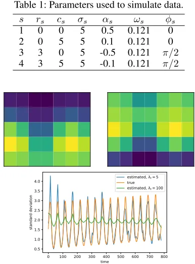
The variance at each time and location is computed as the weighted sum ofKbell-shaped functions where the weights are time-varying, consist of a linear trend and a periodic term. The bell-shaped functions impose spatial smoothness while the linear trend and the periodic terms enforce the temporal smoothness similar to the seasonal component in real climate data. We simulated the data on a 5×7 grid for 780 time steps withK = 4. This yields a small enough problem to be evaluated many times while still mimicking important properties of climate data. Specific parameter choices of the variance function are shown in Table 1. For illustration, we also plot the variance function for all locations att= 25and

Table 1: Parameters used to simulate data.

s rs cs σs αs ωs φs

1 0 0 5 0.5 0.121 0

2 0 5 5 0.1 0.121 0

3 3 0 5 -0.5 0.121 π/2

4 3 5 5 -0.1 0.121 π/2

Figure 2: Top: Variance function att= 25(left) andt= 45

(right). Bottom: The true (orange) and estimated standard deviation function at the location (0,0). The estimated values are obtained using linearized ADMM withλs= 0.1and two

values ofλt:λt= 5(blue) andλt= 100(green).

t = 45(Figure 2, top panel) as well as the variance across time at location(0,0)(Figure 2, bottom panel, orange).

We estimated the linearized ADMM for all combi-nations of values of λt and λs from the sets λt ∈

{0,1,5,10,50,100}and λs ∈ {0,0.05,0.1,0.2,0.3}. For

each pair, we then compute the mean absolute error (MAE) between the estimated variance and the true variance at all locations and all time steps. Forλt= 5andλs= 0.1, the

MAE was minimized. The bottom panel of Figure 2 shows the true and the estimated standard deviation at location (0,0) andλt= 5(blue) andλt= 100(green) (λs= 0.1). Larger

values ofλtlead to estimated values which are “too smooth”.

The left panel of Figure 3 shows the convergence of both Al-gorithms as a function of iteration. It is important to note that each iteration of the linearized algorithm takes 0.01 seconds on average while each iteration of the consensus ADMM takes about 20 seconds. Thus, where the lines meet at 400 iterations requires about 4 seconds for the linearized method and 2 hours for the consensus method. For consensus ADMM, computation per iteration per core requires∼10 seconds with ∼4 seconds for communication. In general, the literature sug-gests linear convergence for ADMM (Nishihara et al. 2015) and Figure 3 seems to fit in the linear framework for both algorithms, though with different constants.

(6)

our method spatial

(t=0) temporal(s=0) GARCH 0.2

0.3 0.4 0.5 0.6 0.7 0.8

MAE

Figure 3: Left: Value of the objective function for linearized (orange) and consensus (blue) ADMM against iteration. Right: MAE for (1) our method with optimal values ofλt

andλs(2) spatial penalty only (3) temporal penalty only and

(4) a GARCH(1,1).

not consider the spatial smoothness (equivalent to fitting the model in Section 2.1 to each time-series separately), a model which only imposes spatial smoothness, and a GARCH(1,1) model. We simulated 100 datasets using the method explained above withσs∼uniform(4,7). The right panel of Figure 3

shows the boxplot of the MAE for these models. As discussed above, using an algorithm akin to (Hallac et al. 2017) ignores the spatial component and thus gives results which are similar to the second column if the covariances are shrunk to zero (massively worse if they are estimated).

4.2 Data Analysis

Consensus ADMM in Section 3.1 is appropriate when we can easily parallelize over multiple machines. Otherwise, it is significantly slower, so all the results reported in this section are obtained using Algorithm 2. We applied this algorithm to the Northern Hemisphere of the ERA-20C dataset avail-able from the European Center for Medium-Range Weather Forecasts4. We use the 2 meter temperature measured daily at noon local time from January 1, 1960 to December 24, 2010.

Preprocessing and other considerations Examination of the time-series alone demonstrates strong differences be-tween trend and cyclic behavior across spatial locations (the data are not mean-zero). One might try to model the cycles by the summation of sinusoidal terms with different frequen-cies. However, for some locations, this would require many frequencies to achieve a reasonable level of accuracy, while other locations would require relatively few. In addition, such a model cannot capture the non-stationarity in the cycles.

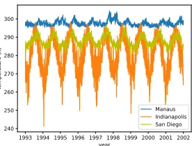
Figure 4 shows the time-series of the temperature of three cities: Indianapolis (USA), San Diego (USA) and Manaus (Brazil). The time-series of Indianapolis and San Diego show clear cyclic behavior, though the amplitude is different. The time-series of Manaus does not show any regular cyclic be-havior. For this reason, we first apply trend filtering to remove seasonal terms and detrend every series. For each time-series, we found the optimal value of the penalty parameter using 5-fold cross-validation.

The blue curve in the top panel of Figure 5 shows the daily temperature for Indianapolis after detrending. The red

4

https://www.ecmwf.int

Figure 4: Time-series of the temperature (in Kelvin) of three cities.

Figure 5: Top: The variability of the time-series of Indianapo-lis (weekly) and the estimated SD obtained from the method of Section 2.1 (red). Lower left: the estimated SDs (red) and their annual average (black) without the long horizon penalty. Lower right: the same but with the long horizon penalty.

curve shows the estimated SD,exp(ht/2), obtained from

our proposed model. For ease of analysis, we compute the average of the estimated SD for each year. Both are shown in the lower left panel of Figure 5.

In addition to the constraints discussed in Section 2.2, we add a long horizon penalty to smooth the annual trend:

PNyear−1

i=2

P

thA(−1)−2hA(0)+hA(1)

whereNyearis the number of years andA(b) ={t:t∈(year_i+b)}. Finally, because the observations are on the surface of a hemisphere rather than a grid, we add extra spatial constraints with the obvious form to handle the boundary between180◦W and

180◦E as well as the region near the North Pole. The esti-mated SDs for Indianapolis are shown in the lower right panel of Figure 5. The annual average of the estimated SDs shows a linear trend with a positive slope.

As shown in Algorithm 2, we checked convergence using

= 0.001%of the MSE of the data. Our simulations indi-cated that the convergence speed depends on the value ofλt

andλs. For the temperature data, we used the solutions

(7)

1961 1971 1981 1991 2001 2011 10

5 0 5 10

1961 1971 1981 1991 2001 2011 10

5 0 5 10

data estimated SD yearly average of estimated SD

year

te

m

p

e

ra

tu

re

(

K

)

D

if

fe

re

nc

e

in

tr

en

d

(K

)

year

1961 1971 1981 1991 2001 2011 10

5 0 5 10

1961 1971 1981 1991 2001 2011 10

5 0 5 10

data estimated SD yearly average of estimated SD

year

te

m

p

e

ra

tu

re

(

K

)

D

if

fe

re

nc

e

in

tr

en

d

(K

)

year

Figure 6: Residuals from the estimated trend (blue), the es-timated SDs (orange), and annual average SD (green) for Indianapolis (left) and San Diego (right). Units are K◦.

for larger values. Estimation takes between 1 and 4 hours for convergence for each pair of tuning parameters.

Model Selection One common method for choosing the penalty parameters in lasso problems is to find the solution for a range of the values of these parameters and then choose the values which minimize a model selection criterion. However, such analysis needs either the computation of the degrees of freedom or requires cross validation. Previous work has investigated the degrees of freedom in generalized lasso prob-lems with Gaussian likelihood (Tibshirani and Taylor 2012; Hu, Zeng, and Lin 2015; Zeng, Hu, and Li 2017), but, re-sults for non-Gaussian likelihood remains an open problem, and cross validation is too expensive. In this paper, there-fore, we use a heuristic method for choosingλtandλs: we

compute the solutions for a range of values of and choose those which minimizeL(λt, λs) =−l(y|h) +PkDhk. This

objective is a compromise between the negative log like-lihood and the complexity of the solution. For smoother solutions the value of P_k_Dh_k _{will be smaller but with}

the cost of larger −l(y|h). We computed the solution for all the combinations of the following sets of values:λt ∈

{0,2,4,8,10,15,200,1000}, λs∈ {0, .1, .5,2,5,10}. The

best combination wasλt= 4andλs= 2.

Analysis of Trends in Temperature Volatility Figure 6 shows the detrended data, the estimated standard deviation and the yearly average of these estimates for two cities in the US: Indianapolis (left) and San Diego (right). The estimated SD captures the periodic behavior in the variance of the time-series. In addition, the number of linear segments changes adaptively in each time window depending on how fast the variance is changing.

The yearly average of the estimated SD captures the trend in the temperature volatility. For example, we can see that the variance in Indianapolis displays a small positive trend (easiest to see in Figure 5). To determine how the volatil-ity has changed in each location, we subtract the average of the estimated variance in 1961 from the average in the following years and compute their sum. The average esti-mated variance at each location is shown in the top panel of Figure 7 while the change from 1961 is depicted in bot-tom panel. Since the optimal value of the spatial penalty is rather large (λs= 2) the estimated variance is spatially very

smooth.

Figure 7: The average of the detrended estimated variance over the northern hemisphere (top) and the change in the variance from 1961 to 2011 (bottom). Units are K◦.

The SD in most locations on the northern hemisphere had a negative trend in this time period, though spatially, this decreasing pattern is localized mainly toward the extreme northern latitudes and over oceans. In many ways, this is consistent with climate change predictions: oceans tend to operate as a local thermostat, regulating deviations in local temperature, while warming polar regions display fewer days of extreme cold. The most positive trend can be observed in Asia, particularly South-East Asia.

5 Discussion

In this paper, we proposed a new method for estimating the variance of spatio-temporal data with the goal of analyzing global temperatures. The main idea is to cast this problem as a constrained optimization problem where the constraints en-force smooth changes in the variance for neighboring points in time and space. In particular, the solution is piecewise linear in time and piecewise constant in space. The result-ing optimization is in the form of a generalized LASSO problem with high-dimension, and so applying the PDIP method directly is infeasible. We therefore developed two ADMM-based algorithms to solve this problem: the consen-sus ADMM and linearized ADMM.

(8)

Acknowledgements

This material is based upon work supported by the National Science Foundation under Grant Nos. DMS–1407439 and DMS–1753171.

References

Andersen, M. S.; Dahl, J.; and Vandenberghe, L. 2013.CVXOPT: A Python package for convex optimization, version 1.1.6.Available

atcvxopt.org.

Bender, F. A.; Ramanathan, V.; and Tselioudis, G. 2012. Changes in extratropical storm track cloudiness 1983–2008: Observational support for a poleward shift. Climate Dynamics38(9-10):2037– 2053.

Besag, J. 1974. Spatial interaction and the statistical analysis of lattice systems. Journal of the Royal Statistical Society. Series B (Methodological)36:192–236.

Bony, S.; Stevens, B.; Frierson, D. M.; Jakob, C.; Kageyama, M.; Pincus, R.; Shepherd, T. G.; Sherwood, S. C.; Siebesma, A. P.; Sobel, A. H.; et al. 2015. Clouds, circulation and climate sensitivity.

Nature Geoscience8(4):261.

Boucher, O.; Randall, D.; Artaxo, P.; et al. 2013. Clouds and aerosols. In Stocker, T.; Qin, D.; Plattner, G.-K.; et al., eds.,Climate Change 2013: The Physical Science Basis. Contribution of Working Group I to the Fifth Assessment Report of the Intergovernmental Panel on Climate Change. Cambridge University Press. 571–657. Boyd, S.; Parikh, N.; Chu, E.; Peleato, B.; and Eckstein, J. 2011. Distributed Optimization and Statistical Learning via the Alternat-ing Direction Method of Multipliers. Foundations and Trends in Machine Learning3(1):1–122.

Corless, R. M.; Gonnet, G. H.; Hare, D. E. G.; Jeffrey, D. J.; and Knuth, D. E. 1996. On the LambertW function. Advances in Computational Mathematics5(1):329–359.

Engle, R. 2002. Dynamic conditional correlation: A simple class of multivariate generalized autoregressive conditional heteroskedastic-ity models.Journal of Business & Economic Statistics20(3):339– 350.

Fischer, E. M.; Beyerle, U.; and Knutti, R. 2013. Robust spatially aggregated projections of climate extremes.Nature Climate Change

3:1033—1038.

Gibberd, A. J., and Nelson, J. D. 2017. Regularized estimation of piecewise constant gaussian graphical models: The group-fused graphical lasso.Journal of Computational and Graphical Statistics

26(3):623–634.

Grise, K. M.; Polvani, L. M.; Tselioudis, G.; Wu, Y.; and Zelinka, M. D. 2013. The ozone hole indirect effect: Cloud-radiative anoma-lies accompanying the poleward shift of the eddy-driven jet in the southern hemisphere.Geophysical Research Letters40(14):3688– 3692.

Hallac, D.; Park, Y.; Boyd, S.; and Leskovec, J. 2017. Network inference via the time-varying graphical lasso. InProceedings of the 23rd ACM SIGKDD International Conference on Knowledge Discovery and Data Mining, KDD ’17, 205–213. New York, NY, USA: ACM.

Hansen, J.; Sato, M.; and Ruedy, R. 2012. Perception of climate change.Proceedings of the National Academy of Sciences109(37). Harvey, A.; Ruiz, E.; and Shephard, N. 1994. Multivariate stochastic variance models.The Review of Economic Studies61(2):247–264. Hu, Q.; Zeng, P.; and Lin, L. 2015. The dual and degrees of freedom of linearly constrained generalized lasso.Computational Statistics & Data Analysis86:13–26.

Huntingford, C.; Jones, P. D.; Livina, V. N.; Lenton, T. M.; and Cox, P. M. 2013. No increase in global temperature variability despite changing regional patterns.Nature500(7462):327–330.

Kahn, B. H.; Fishbein, E.; Nasiri, S. L.; Eldering, A.; Fetzer, E. J.; Garay, M. J.; and Lee, S.-Y. 2007. The radiative consistency of atmospheric infrared sounder and moderate resolution imaging spec-troradiometer cloud retrievals. Journal of Geophysical Research: Atmospheres112(D9).

Kim, S.-J.; Koh, K.; Boyd, S.; and Gorinevsky, D. 2009. `1trend filtering.SIAM Review51(2):339–360.

Monti, R. P.; Hellyer, P.; Sharp, D.; Leech, R.; Anagnostopoulos, C.; and Montana, G. 2014. Estimating time-varying brain connectivity networks from functional MRI time series.NeuroImage103:427– 443.

Myers, T. A.; Mechoso, C. R.; and DeFlorio, M. J. 2018. Importance of positive cloud feedback for tropical atlantic interhemispheric climate variability.Climate Dynamics51(5-6):1707–1717. Nishihara, R.; Lessard, L.; Recht, B.; Packard, A.; and Jordan, M. 2015. A general analysis of the convergence of admm. In Bach, F., and Blei, D., eds.,Proceedings of the 32nd International Conference on Machine Learning, volume 37, 343–352. PMLR.

Parikh, N., and Boyd, S. 2014. Proximal Algorithms.Foundations and TrendsR in Optimization1(3):127–239.

Rhines, A., and Huybers, P. 2013. Frequent summer temperature extremes reflect changes in the mean, not the variance.Proceedings of the National Academy of Sciences110(7):E546–E546.

Schreier, M.; Kahn, B.; Eldering, A.; Elliott, D.; Fishbein, E.; Irion, F.; and Pagano, T. 2010. Radiance comparisons of modis and airs using spatial response information. Journal of Atmospheric and Oceanic Technology27(8):1331–1342.

Screen, J. A. 2014. Arctic amplification decreases temperature variance in northern mid- to high-latitudes.Nature Climate Change

4:577—582.

Staten, P. W.; Kahn, B. H.; Schreier, M. M.; and Heidinger, A. K. 2016. Subpixel characterization of HIRS spectral radiances using cloud properties from AVHRR.Journal of Atmospheric and Oceanic Technology33(7):1519–1538.

Tibshirani, R. J., and Taylor, J. 2012. Degrees of freedom in lasso problems. The Annals of Statistics40(2):1198–1232.

Tibshirani, R. J. 2014. Adaptive piecewise polynomial estimation via trend filtering.Annals of Statistics42:285–323.

Trenberth, K. E.; Zhang, Y.; Fasullo, J. T.; and Taguchi, S. 2014. Climate variability and relationships between top-of-atmosphere ra-diation and temperatures on earth.Journal of Geophysical Research: Atmospheres120(9):3642–3659.

Vasseur, D. A.; DeLong, J. P.; Gilbert, B.; Greig, H. S.; Harley, C. D. G.; McCann, K. S.; Savage, V.; Tunney, T. D.; and O’Connor, M. I. 2014. Increased temperature variation poses a greater risk to species than climate warming.Proceedings of the Royal Society of London B: Biological Sciences281(1779).

Wang, Y.-X.; Sharpnack, J.; Smola, A. J.; and Tibshirani, R. J. 2016. Trend filtering on graphs.Journal of Machine Learning Research

17(105):1–41.

Wielicki, B. A.; Young, D.; Mlynczak, M.; Thome, K.; Leroy, S.; Corliss, J.; Anderson, J.; Ao, C.; Bantges, R.; Best, F.; et al. 2013. Achieving climate change absolute accuracy in orbit.Bulletin of the American Meteorological Society94(10):1519–1539.