Multilevel preconditioners for embedded enriched partition of unity approximations

R E S E A R C H A R T I C L E

Open Access

Multilevel preconditioners for embedded

enriched partition of unity approximations

Marc Alexander Schweitzer

and Albert Ziegenhagel

*_{Correspondence:}

[email protected] 1_{Fraunhofer-Institut für}

Algorithmen und Wissenschaftliches Rechnen SCAI, Schloss Birlinghoven, 53757 Sankt Augustin, Germany Full list of author information is available at the end of the article

Abstract

In this paper we are concerned with the non-invasive embedding of enriched partition of unity approximations in classical finite element simulations and the efficient solution of the resulting linear systems. The employed embedding is based on the partition of unity approach introduced in Schweitzer and Ziegenhagel (Embedding enriched partition of unity approximations in finite element simulations. In: Griebel M, Schweitzer MA, editors. Meshfree methods for partial differential equations VIII. Lecture notes in

science and engineering, Cham, Springer International Publishing; 195–204,2017)

which is applicable to any finite element implementation and thus allows for a stable enrichment of e.g. commercial finite element software to improve the quality of its approximation properties in a non-invasive fashion. The major remaining challenge is the efficient solution of the arising linear systems. To this end, we apply classical subspace correction techniques to design non-invasive efficient multilevel solvers by blending a non-invasive algebraic multigrid method (applied to the finite element components) with a (geometric) multilevel solver (Griebel and Schweitzer in SIAM J Sci

Comput 24:377–409,2002; Schweitzer in Numer Math 118:307–28,2011) (applied to

the enriched embedded components). We present first numerical results in two and three space dimensions which clearly show the (close to) optimal performance of the proposed solver.

Keywords: Partition of unity method, Generalized finite element method, Multilevel solver, Subspace correction, Domain decompositon

Mathematics Subject Classification: Primary 65N55, 65N30

Introduction

The direct generalization and extension of the classical finite element method (FEM) to allow for the use of arbitrary non-polynomial basis functions as in partition of unity (PU) based approaches like XFEM/GFEM [1–5] usually requires a fair amount of implemen-tational work within the original finite element (FE) code. Thus, the timely evaluation of novel generalizations of the FEM in large-scale industrial applications, which in general rely on commercial software packages, is usually not feasible. This issue can, however, be overcome with the help of the embedding approach presented in [6]. It allows for the non-invasive stable embedding of an arbitrary approximation spaceVENRinto a classical FE spaceVHOSTand thereby enables the easy evaluation of novel generalizations of the FEM empolying arbitrary approximation functions in an industrial context. In [6] it was demonstrated that the approach is free from artifacts and yields substantial improvements

©The Author(s) 2018. This article is distributed under the terms of the Creative Commons Attribution 4.0 International License (http://creativecommons.org/licenses/by/4.0/), which permits unrestricted use, distribution, and reproduction in any medium, provided you give appropriate credit to the original author(s) and the source, provide a link to the Creative Commons license, and indicate if changes were made.

in terms of accuracy. Note that this approach is very different from classical global–local techniques where you consider an independent auxilliary local problem. We, however, blend two function spacesVHOSTandVENRto discretize the global problem directly with a single larger function space VBND which comprisesVHOST andVENR, compare also [7–9].

In this paper we are concerned with the construction of highly efficient solvers and preconditioners for the linear system arising from the discretization of the global prob-lem with this blended function space VBND. To this end, we are concerned with the non-invasive construction of multilevel preconditioners based on subspace correction methods [10] which are also referred to as Schwarz methods e.g. in the domain decom-position context [11]. We construct the coarsening process forVBNDwith the help of an available (geometric) multilevel structure ofVENRand a multilevel decomposition of VHOSTobtained by an algebraic multigrid (AMG) method in a non-invasive fashion. The remainder of this paper is structured as follows: we first quickly introduce the mathemat-ical foundation of our embedding approach, the partition of unity method (PUM), in “A partition of unity method for the embedding of arbitrary approximation spaces in finite element spaces” and summarize the actual embedding procedure. In “Subspace correc-tion methods” we introduce efficient subspace correccorrec-tions precondicorrec-tioners for the linear system arising from the discretization of the global problem by our blended function space VBND. The results of our numerical experiments with these preconditioners are presented in “Numerical results” before we conclude with some remarks in “Concluding remarks”.

A partition of unity method for the embedding of arbitrary approximation spaces in finite element spaces

The PUM was introduced in [1,12] as a generalization of the FEM and is based on [13]. The abstract ingredients which make up a PUM space

VPU:=

N

i=1

ϕiVi=spanϕiϑim; (1)

are a partition of unity (PU){ϕi :i = 1,. . ., N}and a collection of local approximation spaces Vi := Vi(ωi) := spanϑ_im

d_Vi

m=1defined on the patches ωi := supp(ϕi) fori = 1,. . ., N. Thus, the shape functions of a PUM space are simply defined as the products of the PU functionsϕiand the local approximation functionsϑim. The PU functions provide the locality and global regularity of the product functionsϕiϑim whereas the functions

ϑm

ΩENR,FT

ΩHOST,FT

ΩΦ

ΓD ΓN

ΓD

ΓN

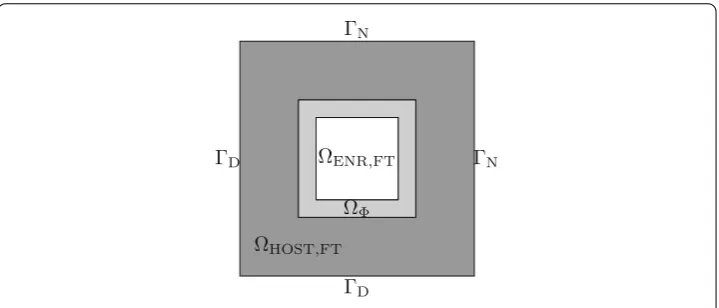
Fig. 1 Sketch of smooth model problem in two dimensions depicting the employed partitioning of the domainintoHOST,FT(drak gray),=HOST∩ENR(light gray), andENR,FT(white). The boundary data

for this model problem is given byg=0 onDandh=(1,1)T·nonNwherendenotes the outer normal

Let us consider a very simple cover of the domaininto just two overlapping patches (or subdomains)0and1with respective PU functions0and1, i.e.0+1≡1 on

⊆ 0∪1. Then, let us choose the approximation spaceV0on the patch0to be a classical FE space defined on a respective mesh0,hwhich discretizes0. According to the general PUM approximation theory this choice ofV0imposes absolutely no constraints on our choice of the approximation spaceV1on the other subdomain1. For instance, we could choose another FE space on a non-matching mesh1,Hand blend these non-matching spaces smoothly together via the PUM [7,8]. Another admissible choice forV1 is the use of a locally enriched PUM space [6]. Throughout this paper we focus on the latter case where we blend an enriched approximation space with a classical FE space. Thereby, we can equip any classical FE simulation with stable enrichment capabilities via the PUM in a non-invasive fashion. To this end, let us introduce some more descriptive notation to identify the various components employed in our overall scheme. We refer to the two patches or subdomains byHOSTandENR, compare Fig.1. Moreover, we denote the respective function spaces defined on these subdomains byVHOSTandVENRwhere VHOSTis a classical FE space andVENRis an enriched approximation space. Note that in this simplistic two subdomain case we can rewrite the PU functions asHOST:=and

ENR:=(1−) with some non-negative weight functionwith supp()=¯HOST. With the help of this notation and (1) we define our blended global approximation space VBNDon the complete domainby

VBND:=HOSTVHOST+ENRVENR=VHOST+(1−)VENR (2)

such that any elementv∈VBNDcan be written as

vBND=HOSTvHOST+ENRvENR

with vHOST ∈ VHOSTandvENR ∈ VENR. Note that the general convergence theory of the PUM [1,12] allows to obtain some straightforward error bounds for this blending approach. To this end, let us consider the following estimate from [14].

Theorem 1 Let⊂RDbe a Lipschitz domain. Let{ϕi :i=1,. . ., N}be an admissible

Let us further introduce the covering indexλC :→Nsuch that

λC(x) :=card({ωi∈C:x∈ωi}) (3)

and let us assume that

λC(x)≤ ∈N for all x∈ (4)

with independent of the number of patches N . Let a collection of local approximation spaces Vi = spanϑ_im ⊂ H1(ωi)be given. Let f ∈H1()be the function to be

approxi-mated. Assume that the local approximation spaces Vihave the following approximation

properties: On each patch∩ωi, the function f can be approximated by a function vi∈Vi

such that

f −viL2_(∩ωi)≤ˆi, and ∇(f −vi)L2_(∩ωi)≤˜i (5)

hold for all i=1,. . ., N . Then the function

v:=

N

i=1

ϕivi∈VPU⊂H1()

satisfies the global estimates

f −v_L2₍₎≤

_N

i=1

ϕiL∞(Rd₎ˆ2_i

1/2

, (6)

∇(f −v)_L2₍₎≤

√ 2

_N

i=1

∇ϕiL∞(Rd₎ˆi 2

+ ϕiL∞(Rd₎˜_i2

1/2

. (7)

In our setting we only have two approximation spacesVHOSTandVENRand let us, for the ease of notation, assume that both spaces (i= HOST,ENR) admit error bounds (5) of the form

f −viL2_(∩ωi)≤Chp_HOST+1 , and ∇(f −vi)L2_(∩ωi)≤Chp_HOST. (8)

Then it is sufficient to ensure that the estimates

∇L∞(Rd₎≤

C_∇ hHOST

, _L∞_(Rd₎≤C∞

are satisfied by our PU functionto attain optimal convergence with the blended function space. Thus, our blending by the PUM provides optimal convergence even for very small overlap regionsHOST∩ENR.

The Galerkin discretization of a partial differential equation (PDE) using this blended function spaceVBNDyields the linear system

KBNDuBND˜ =fBND,ˆ (9)

where ˆfBND denotes the load vector and ˜uBND the respective coefficient vector of the solution. If we assume that the PU functionsatisfies the so-called flat-top property

for some subsetHOST,FT ⊂ HOST=HOST,FT∪with:= HOST\HOST,FT. Obviously, the other PU function (1−)=ENRthen satisfies

(1−)|_ENR,FT=ENR|ENR,FT≡1

for someENR,FT ⊂ENR=ENR,FT∪withHOST,FT∩ENR,FT= ∅andHOST∩

ENR=. With the help of the flat-top property of the PU we can thus introduce the splitting

VBND:=VHOST,FT+HOSTVHOST⊥ ,FT+ENRVENR⊥ ,FT+VENR,FT (10)

of our global blended function spaceVBNDinto four components where anyv∈VHOST,FT satisfies supp(v) ⊂ ¯HOST,FT and V_HOST⊥ _,FT denotes the complement of VHOST,FT in VHOST. The respective block-partitioning of the global stiffness matrix then reads as

KBND= ⎛ ⎜ ⎜ ⎜ ⎝

KHF,HF KHF,HF⊥ 0 0

K_HF⊥_,HFK_HF⊥_,HF⊥ K_HF⊥_,EF⊥ 0 0 K_EF⊥_,HF⊥ K_EF⊥_,EF⊥ K_EF⊥_,EF 0 0 K_EF,EF⊥ KEF,EF

⎞ ⎟ ⎟ ⎟

⎠. (11)

The load vector ˆfBNDand coefficient vector ˜uBNDin this block-form are given by

ˆ fBND=

⎛ ⎜ ⎜ ⎜ ⎝ ˆ fHF ˆ f_HF⊥

ˆ f_EF⊥

ˆ fEF ⎞ ⎟ ⎟ ⎟

⎠ and u˜BND= ⎛ ⎜ ⎜ ⎜ ⎝ ˜ uHF ˜ u_HF⊥

˜ u_EF⊥

˜ uEF ⎞ ⎟ ⎟ ⎟ ⎠.

Note that the sub-matrix KHF,HFis the classical FE stiffness matrix on the sub-domain

HOST,FT and thus can be provided by any FE package whereas all other sub-matrices in (11) need to be computed by the embedding code. Hence, our approach is completely non-invasive to a (commercial) FE package with respect to the disjoint partitioning of the domainintoHOST,FT⊂, which is discretized by the (commerical) FE package, and\HOST,FT, compare Fig.1. However, we actually employ a FE discretization on

HOST=HOST,FT∪which is obtained by merging the FE discretization onHOST,FT provided by the HOST code and the discretization on provided by our embedding code, see [6] for details. Obviously, the overall computational effort associated with the assembly of the linear system (9) thus scales with the size of the overlap region and thus a small overlap region is preferable from this point of view.

Considering the disjoint partitioning of the domainintoHOST,FT,andENR,FT we can introduce the block-partitioning

KBND= ⎛ ⎜ ⎝

KHF,HFKHF, 0

K,HF K, K,EF 0 KEF, KEF,EF

⎞ ⎟

⎠, (12)

where

K,:=

K_HF⊥_,HF⊥ K_HF⊥_,EF⊥

K_EF⊥_,HF⊥ K_EF⊥_,EF⊥

,

construction of multigrid-like solvers for (9) via the blending of respective multilevel sequences ofVHOSTandVENRand thus employ the even more compact block-partitioning

KBND=

KH,HKH,E KE,H KE,E

, fBNDˆ =

ˆ fH

ˆ fE

, uBND˜ =

˜ uH

˜ uE

, (13)

where

KH,H:=

KHF,HF KHF,HF⊥ K_HF⊥_,HFK_HF⊥_,HF⊥

.

Note, however, that this disjoint partitioning of the matrix corresponds to an overlapping partitioning of the domainintoHOST=HOST,FT∪andENR=ENR,FT∪. To introduce our proposed multilevel solver for (9) based on the partitioning (13) let us shortly review the general components of such solvers in the context of subspace correction methods.

Subspace correction methods

The computational effort associated with the solution of linear systems like (9) account for a very large part (often even the largest) of the overall computational cost in any implicit or stationary simulation. Thus, the development of efficient linear solvers is of great practical relevance and is still an active research field today. Even though classical general purpose numerical linear algebra techniques such as (sparse) matrix factorizations, see e.g. [15], are widely used in practice, it is well-known that their computational complexity is not optimal and that specialized iterative linear solvers are needed to tackle large scale problems with millions of unknowns efficiently.

A very sophisticated class of iterative methods which not only show an optimal scaling in the storage demand but also in the operation count are so-called multilevel iterative solvers or (geometric) multigrid methods which are particular instances of subspace cor-rection methods [10]. Note, however, that these multilevel and multigrid solvers are not general algebraic methods but involve a substantial amount of information about the dis-cretization and possibly the PDE. Thus, the introduction of such a (geometric) multilevel solver in a commercial software package is very much invasive and typically infeasible. However, there exist extensions of (geometric) multigrid methods, so-called algebraic multigrid methods (AMG) [16–19], which can be used as a non-invasive plugin solver also in commercial software [20,21]. Such AMG solvers are successfully utilized in many different application fields yet they are essentially designed for classical mesh-based piece-wise linear discretizations and thus are in general not directly applicable to discretizations with arbitrary approximation functions, i.e.VBNDandVENR. Therefore, no optimal linear solver for (9) is readily available and we need to take the specific construction of our blended approximation spaceVBNDinto account when designing a respective iterative linear solver. To this end, we employ classical subspace correction techniques which can utilize splittings such as (2) and (10).

V =

J

i=0

Vi (14)

of a global function spaceV, the PSC iteration reads

˜ u←u˜+

J

i=0

Bi(ˆf −Ku˜) (15)

with

Bi :=PiK_i−1PiT, the prolongation Pi:Vi→V, (16)

and Ki denoting the stiffness matrix with respect to subspace Vi. The SSC scheme is defined by

Fori=0,. . ., J : u˜←u˜+Bi(ˆf −Ku˜) (17)

and thus involves a successive update of the residual ˆf−Ku˜after each subspace correction. Note that the use of the exact inverseK_i−1in (16) is not necessary. In fact, the use of approximate subspace solvers is usually advisable and much more common, i.e. we define

Bi :=PiWiPiT with Wi≈Ki−1. (18)

The main ingredients which control the performance of the iterations (15) and (17) are the specific choices of the subspace splitting (14), the prolongations (16) and the approximate subspace solversWi in (18) where it is important to note that we do not assume that (14) allows for a unique decompositionv = J_i=0vi of a functionv ∈ V. In fact, the redundancy in the splitting (14) has a substantial impact on the convergence properties of (15) and (17).

In classical multigrid terminology the approximate subspace solvers Wi in (18) are referred to as smoothers and the subspacesVicorrespond to the employed approximation spaces defined on different refinement levels of the underlying mesh, i.e. VJ =Vdenotes the finest discretization space andViwithi<Jare referred to as coarse spaces. The role of the smoothersWiis to reduce high frequency error components whereas the corrections

Bi(ˆf −Ku˜) obtained on the coarser levels should reduce low frequency errors so that all error frequencies are efficiently reduced in each iteration.

In the following we first focus on the construction of the coarse spacesViwithi < J for our finest discretization spaceVJ = V = VBNDand the definition of the respective prolongationsPi:Vi→V =VJ =VBND. To this end, let us review an essential property that the prolongationsPiand coarse spacesVishould satisfy. Since the role of the coarse spacesViis the resolution of low frequency errors they should at least contain the constant functions, i.e. 1 ∈Vi, and the prolongations should be exact for the constant functions. Thus, we need to specify a coarsening process for the blended space VBND = VJ such that the resulting coarse space VJ−1 contains constants and a respective prolongation PJ−1 : VJ−1 → VJ = VBNDwhich preserves constants. To this end, let us consider the representation of the constant functions inVJ =VBND

where 1HOST∈VHOSTand 1ENR∈VENRdenote the constant function on the overlapping sub-domains HOST andENR respectively. Therefore, we can localize the coarsening process for the space VBND to the two spacesVHOST and VENR and then define the prolongation as

PJ−1:=

PHOST,J−1 0 0 PENR,J−1

provided that the two prolongationsPHOST,J−1 : VHOST,J−1 → VHOST andPENR,J−1 : VENR,J−1→VENRpreserve constants inVHOSTandVENRrespectively. Hence, let us now focus on the definition of a non-invasive coarsening process forVHOSTwhich comprises the FE spaceVHOST,FT(handled by the HOST code) and the FE spaceV_HOST⊥ _,FTvia AMG techniques.

In general, AMG constructs a suitable coarse spaceVJ−1⊂VJand a respective prolon-gationPJ−1:VJ−1→VJ that preserves constants from the stiffness matrixKJ obtained by the Galerkin discretization of the PDE using the spaceVJ. In our setting, however, the blockKH,Hof the stiffness matrix (13) does not correspond to the Galerkin discretization byVHOSTbut by the spaceHOSTVHOST(which does not contain the constant function). Thus, only the blockKHF,HFof the matrix

KH,H:=

KHF,HF KHF,HF⊥ K_HF⊥_,HFK_HF⊥_,HF⊥

is given by a classical FE discretization and all other blocks are computed using basis functions that are products HOSTφk of our PU functionHOSTand classical FE basis functionsφk. Applying AMG directly toKH,Htherefore does not provide a suitable pro-longation that preserves constants inVHOST, compare Fig.2. To overcome this issue in a way that is non-invasive also to AMG we simply set up an auxiliary matrix

¯ KH,H:=

KHF,HF K¯HF,HF⊥ ¯

K_HF⊥_,HFK¯_HF⊥_,HF⊥

where we exchange the matrix blocks that involveHOSTinKH,Hby their unweighted counterparts, i.e. which are computed using the classical FE basis functionsφkinstead of the productsHOSTφk. The matrix blockKHF,HFis unchanged so that the non-invasive character of our approach to the HOST code is fully maintained and no additional assem-bly on the sub-domainHOST,FT that is handled by the HOST code is necessary. Since

¯

KH,Hnow satisfies all assumptions of AMG, we obtain a suitable coarse spaceVHOST,J−1 and associated prolongation ¯PHOST,J−1from the application of AMG to ¯KH,H, compare Fig. 2. In fact, AMG automatically computes a sequence of coarse spacesVHOST,i and associated prolongations ¯Pi

HOST,i−1:VHOST,i−1→VHOST,i.

For the embedded spaceVENR, which in our case is itself a PUM space, we construct a sequence of suitable prolongations ¯Pi_ENR,i−1 : VENR,i−1 →VENR,idirectly by so-called global-to-localL2-projections [22,23] based on a geometric coarsening process. Thus, we can now define a sequence of prolongations

Pi_i−1:=

¯

P_HOSTi _,i−1 0 0 P¯_ENRi _,i−1

and respective coarser versionsKBND,iof our overall stiffness matrixKBND= KBND,J by the so-called Galerkin operators

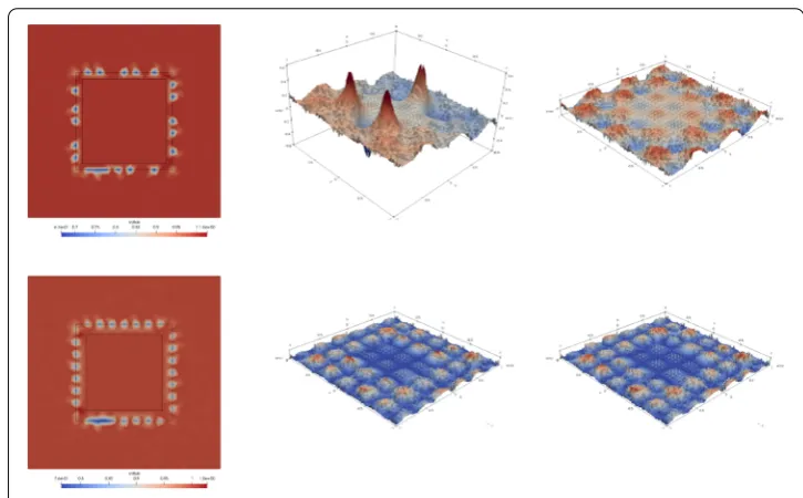
Fig. 2 Contour plots of the prolongation errors (left) attained for the constant function when using the weighted spaceHOSTVHOSTin the AMG construction of the prolongationPJHOST,J−1for a small (top) and a

large overlap region (bottom). Surface plots of the prolongation error of the smooth function sin(3πx) cos(3πy) usingP_HOSTJ _,J−1(center) and ¯PJ_HOST,J−1(right)

Note, however, that this overall coarsening process in fact coarsens the two componentes VHOST andVENR independently and thus may not be optimal on the overlap region

=HOST∩ENRwhere the two spaces interact substantially. Therefore, the overall performance of the proposed scheme will be affected somewhat by the absolute size of the overlap region. Unlike in classical domain decomposition methods where larger overlap yields a convergence improvement, we, however, anticipate that an increasing overlap will rather worsen the convergence behavior since our independent coarsening process then ignores stronger interactions between the spaces.

As a final component we need to specify the approximate subspace solvers or smoothers on the resulting coarse spacesVBND,ito instantiate the iterations (15) and (17). In the fol-lowing we focus on iterations of the form (17), in particular we employ the classical multi-grid iterationMν1,ν2

γ given in Algorithm 3.1 and consider different numbers of smoothing stepsν=ν1=ν2as well as theV-cycle (γ =1) and theW-cycle (γ =2).

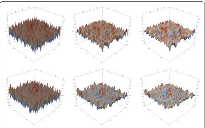
Fig. 3 Surface plots of iterates of a Gauß–Seidel smoother for iteration 1,3,5 (left to right) using a random initial guess on a blended discretization using a small (top) and a large overlap region (bottom)

Numerical results

In this section we present some results of our numerical experiments using the embedded enriched PUM within a classical FE simulation as discussed above. To this end, we consider a set of isotropic model problems focussing on the optimality of the proposed solver only. A detailed study of the solvers robustness with respect to varying material coefficients is the subject of future research. In particular, we are concerned with the approximation of the Poisson problem

−u=f in⊂Rd,

u=g onD⊂∂,

∂u

∂n =h onN =∂\D,

(19)

in two space dimensions on a square domain, see Fig. 1, where we embed a smooth enrichment spaceVENRto identify the best performance of our proposed solver. Then, we consider a non-convex domain, see Fig.4, where we embed an enrichment spaceVENR that contains singular functions to efficiently resolve the corner singularity. Finally, we consider a linearly elastic bar in three space dimensions, see Fig.5, i.e.

−divσ(u)=0 in⊂Rd,

u= g onD ⊂∂, σ(u)· n=0 onC,

σ(u)· n= h onN =∂\D,

(20)

ΩENR,FT

ΩHOST,FT

ΩΦ

ΓN

ΓN

ΓN

ΓN

ΓD

ΓD

Fig. 4 Sketch of a non-convex domainin two dimensions depicting the employed partitioning into

HOST,FT(drak gray),=HOST∩ENR(light gray), andENR,FT(white). The boundary data for this model

problem is given byg=0 onDandh= ∇

(x2+xy+y2+1)(r23sin(2θ−₃π))

·nonNwherendenotes the outer normal

Ω

Ω

Ω

Γ

Γ

Γ

Fig. 5 Sketch of a pre-cracked bar in three dimensions depicting the partitioning of the domaininto

HOST,FT(drak gray),=HOST∩ENR(light gray), andENR,FT(white). The boundary data for this model

problem is given byD=L∪R,g=(0,0,0)TonL,g=(0.02,0,0)TonRandh=(0,0,0)Ton

N=∂\D

employ different embedding configurations with respect to the intersection ofENRwith the boundariesDandN of the global simulation domain, compare Figs.1,4and5.

Fig. 6 Sketch of the blended function discretization space depicting the supports of a basis function

φHOST∈VHOST(light gray) andφENR∈VENR(dark gray). The support sizes are of comparable size throughout

the paper; i.e. diam(supp(φHOST)∼diam(supp(φENR)

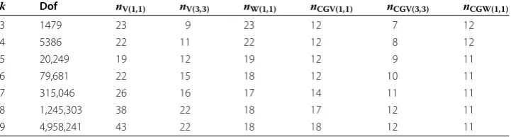
Table 1 Measured iteration numbersnfor the stand-alone solver andnCGfor the preconditioned CG method attained for the model problem (19) on the configuration depicted in Fig.1using a single element overlap

k Dof n_V(1,1) n_V(3,3) n_W(1,1) n_CGV(1,1) n_CGV(3,3) n_CGW(1,1)

3 1479 23 9 23 12 7 12

4 5386 22 11 22 12 8 12

5 20,249 19 12 19 12 9 11

6 79,681 22 15 18 12 10 11

7 315,046 26 16 17 14 11 11

8 1,245,303 38 22 18 17 12 11

9 4,958,241 43 22 18 18 12 11

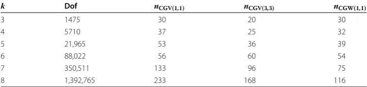
indicating that the quality of the corrections from coarser levels obtained in aV(1, 1)-cycle is somewhat deminished for largerk. Nevertheless, the use of theV(1,1)-cycle as a preconditioner in CG yields fairly stable iteration numbersnCGV(1,1) <20 and provides the fastest time-to-solution for the considered numbers of levelsk. Note that the results summarized in Table1were obtained with a small overlap regionof a single element on the finest level; i.e. the overlap region is in fact shrinking as we refine the discretiza-tion. As mentioned above, we anticipate that for a larger overlap region with fixed volume for all levelsk, i.e. an increasing number of elements in the overlap as we refine, the convergence behavior of the proposed solver will deteriorate somewhat. In fact, the results given in Table2show that the number of iterations increases not only but also grows with larger number of levelskeven when we use the rather expensiveW(1,1)-cycle as a preconditioner in CG. Thus, the results confirm our expectation that it is advisable to choose an overlap regionwhose diameter is proportational to the meshwidth on the finest level employed (unlike in classical domain decomposition approaches) since such a choice yields the least amount of work in the assembly of the blended linear systemKBND and it gives the best solver performance.

0 20 40 10−10

10−4 102 iterations ˆ r 2l

V(1_,1) convergence history

k= 3

k= 4

k= 5

k= 6

k= 7

k= 8

k= 9

0 5 10 15

10−10 10−4 102 iterations ˆ r 2l

CG-_W(1_,1) convergence history

k= 3

k= 4

k= 5

k= 6

k= 7

k= 8

k= 9

Fig. 7 Convergence histories for theV(1,1)-cyle as a stand-alone solver (left) and theW(1,1)-cycle as a preconditioner in CG (right)

Table 2 Measured iteration numbersn_CGfor the preconditioned CG method attained for the model problem (19) on the configuration depicted in Fig.1using a fixed volume overlap

k Dof n_CGV(1,1) n_CGV(3,3) n_CGW(1,1)

3 1475 30 20 30

4 5710 37 25 32

5 21,965 53 36 39

6 88,022 56 60 54

7 350,511 133 96 75

8 1,392,765 233 168 116

let us consider a more relevant case whereVENRcontains problem-dependent singular functions. To this end, we consider (19) on a non-convex domain, see Fig.4. Here, the discretization spaceVENRon the regionENRis defined as

VENR=

N

i=1

ϕi

P1+spanr 2

3 _sin2θ −π

3

(21)

where (r,θ) denote polar coordinates with respect to the re-entrant corner of. Thus, we employ enrichment by a singular function everywhere inENR, see [24] for details on the construction of a stable basis forVENR. Moreover, we use so-called block-Gauß–Seidel relaxation inVENRwhere we collect all degrees of freedom defined on the same patch into a single block, see [22,23] for details. The attained number of iterations are given in Table

3. The overall number of iterations is somewhat larger than in the previous case, however, the number of iterations are essentially independent of the number of levels. It is also noteworthy to point out, that in this model configuration theV(3,3)-cycle substantially outperforms the W(1,1)-cycle which shows the improved smoothing property of the patch-based block-Gauß–Seidel relaxation in VENR. Nevertheless, the fastest time-to-solution for the considered discretizations with more than 13 million degrees of freedom is still obtained by CG preconditioned byV(1,1)-cycle which of course also benefits from the improved smoothing property.

Table 3 Measured iteration numbersn_CGfor the preconditioned CG method attained for the model problem (19) on the configuration depicted in Fig.4using a single element overlap

k Dof n_CGV(1,1) n_CGV(3,3) n_CGW(1,1)

3 3,843 18 10 18

4 14,063 18 10 18

5 54,408 19 11 18

6 214,527 20 11 19

7 847,974 20 12 19

8 3,372,646 21 14 19

9 13,380,007 22 16 13

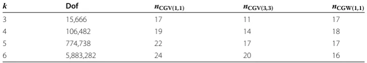
Table 4 Measured iteration numbersnCGfor the preconditioned CG method attained for the model problem (20) on the configuration depicted in Fig.5using a single element overlap

k Dof n_CGV(1,1) n_CGV(3,3) n_CGW(1,1)

3 15,666 17 11 17

4 106,482 19 14 18

5 774,738 22 17 17

6 5,883,282 24 20 16

HOSTand utilize one more layer of bock-partitioning which collects all three displace-ment components in the Gauß–Seidel smoother, i.e. we now use a (3×3)-block relaxation inVHOSTcombined with the block-relaxation inVENRdescribed above. We discretize (20) with trilinear elements inVHOSTand use singular and discontinuous enrichments for the treatment of the crack in VENR (besides linear polynomials). The performance of our proposed solver is summarized in Table4. Again, we find essentially constant iteration numbers for CG preconditioned byW(1,1)-cycle and slightly increasing iteration num-bers when using aV-cycle preconditioner. Yet, the fastest time-to-solution is still attained when using theV(1,1)-cycle as preconditioner.

In summary, the presented results clearly show that the proposed solver yields close to optimal convergence in two and three dimensions when using a small overlap. Using a small overlap is moreover beneficial to the total computational cost in the assembly of the blended linear system and still yields optimal approximation errors.

Concluding remarks

study on the optimal selection of parameters and robustness properties of the proposed scheme is the subject of ongoing and future research.

Authors’ contributions

MAS and AZ developed the method. AZ implemented the method and conducted the numerical experiments. All authors read and approved the final manuscript.

Author details

1_{Fraunhofer-Institut für Algorithmen und Wissenschaftliches Rechnen SCAI, Schloss Birlinghoven, 53757 Sankt Augustin,} Germany,2_{Institut für Numerische Simulation, Rheinische Friedrich-Wilhelms-Universität Bonn, Wegelerstr. 6, 53115} Bonn, Germany.

Acknowledgements Not applicable.

Competing interests

The authors declare that they have no competing interests.

Availability of data and materials Not applicable.

Consent for publication Not applicable.

Ethics approval and consent to participate Not applicable.

Funding Not applicable.

Publisher’s Note

Springer Nature remains neutral with regard to jurisdictional claims in published maps and institutional affiliations.

Received: 9 January 2018 Accepted: 30 April 2018

References

1. Babuška I, Melenk JM. The partition of unity method. Int J Numer Methods Eng. 1997;40:727–58.

2. Belytschko T, Black T. Elastic crack growth in finite elements with minimal remeshing. Int J Numer Methods Eng. 1999;45:601–20.

3. Duarte CA, Oden JT. An hp adaptive method using clouds. Comput Methods Appl Mech Eng. 1996;139:237–62. 4. Fries T-P, Belytschko T. The extended/generalized finite element method: an overview of the method and its

applications. Int J Numer Methods Eng. 2010;84:253–304.

5. Schweitzer M. Variational mass lumping in the partition of unity method. SIAM J Sci Comput. 2013;35:A1073–97. 6. Schweitzer MA, Ziegenhagel A. Embedding enriched partition of unity approximations in finite element simulations.

In: Griebel M, Schweitzer MA, editors. Meshfree methods for partial differential equations VIII., Lecture notes in science and engineeringCham: Springer International Publishing; 2017. p. 195–204.

7. Bacuta C, Xu J. Partition of unity for the Stokes problem on nonmatching grids. In: Proceedings of the 2003 copper mountain conference on multigrid. 2003.

8. Bakuta C, Chen J, Huang Y, Xu J, Zikatanov L. Partition of unity method on nonmatching grids for the Stokes problem. J Numer Math. 2005;13:157–69.

9. Gupta P, Pereira J, Kim D-J, Duarte C, Eason T. Analysis of three-dimensional fracture mechanics problems: a non-intrusive approach using a generalized finite element method. Eng Fract Mech. 2012;90:41–64. 10. Xu J. Iterative methods by space decomposition and subspace correction. SIAM Rev. 1992;34:581–613.

11. Smith BF, Bjørstad PE, Gropp WD. Domain decomposition: parallel multilevel methods for elliptic partial differential equations. Cambridge: Cambridge University Press; 1996.

12. Babuška I, Melenk JM. The partition of unity finite element method: basic theory and applications. Comput Methods Appl Mech Eng. 1996;139:289–314 (Special Issue on Meshless Methods).

13. Babuška I, Caloz G, Osborn JE. Special finite element methods for a class of second order elliptic problems with rough coefficients. SIAM J Numer Anal. 1994;31:945–81.

14. Schweitzer MA. Generalizations of the finite element method. Cent Eur J Math. 2012;10:3–24.

15. Amestoy PR, Duff IS, Koster J, L’Excellent JY. A fully asynchronous multifrontal solver using distributed dynamic scheduling. SIAM J Matrix Anal Appl. 2001;23:15–41.

16. Brandt A. Algebraic multigrid theory: the symmetric case. Appl Math Comput. 1986;19:23–56.

18. Ruge J, Stüben K. Efficient solution of finite difference and finite element equations. In: Multigrid methods for integral and differential equations (Bristol, vol. 3 of Inst. Math. Appl. Conf. Ser. New Ser.) New York: Oxford Univ. Press; 1983, 1985. p. 169–212.

19. Stüben K. A review of algebraic multigrid. J Comput Appl Math. 2001; 128:281–309. Numerical analysis, Partial differential equations: VII; 2000.

20. SAMG—efficiently solving large linear systems of equations.https://www.scai.fraunhofer.de/en/ business-research-areas/fast-solvers/products/samg.html.

21. Stüben K, Ruge JW, Clees T, Gries S. Algebraic multigrid: from academia to industry. In: Griebel M, Schüller A, Schweitzer MA, editors. Scientific computing and algorithms in industrial simulation—projects and products of Fraunhofer SCAI. Cham: Springer International Publishing; 2017. p. 83–120.

22. Griebel M, Schweitzer MA. A particle-partition of unity method—part III: a multilevel solver. SIAM J Sci Comput. 2002;24:377–409.

23. Schweitzer MA. A parallel multilevel partition of unity method for elliptic partial differential equations., Lecture notes in computational science and engineeringBerlin: Springer; 2003.

24. Schweitzer MA. Stable enrichment and local preconditioning in the particle-partition of unity method. Numer Math. 2011;118:137–70.