R E S E A R C H A R T I C L E
Open Access
Evaluation of a weighting approach for
performing sensitivity analysis after
multiple imputation
Panteha Hayati Rezvan
1, Ian R. White
2, Katherine J. Lee
3,4, John B. Carlin
1,3,4and Julie A. Simpson
1*Abstract
Background:Multiple imputation (MI) is a well-recognised statistical technique for handling missing data. As usually implemented in standard statistical software, MI assumes that data are‘Missing at random’(MAR); an assumption that in many settings is implausible. It is not possible to distinguish whether data are MAR or‘Missing not at random’(MNAR) using the observed data, so it is desirable to discover the impact of departures from the MAR assumption on the MI results by conducting sensitivity analyses. A weighting approach based on a selection model has been proposed for performing MNAR analyses to assess the robustness of results obtained under standard MI to departures from MAR.
Methods:In this article, we use simulation to evaluate the weighting approach as a method for exploring possible departures from MAR, with missingness in a single variable, where the parameters of interest are the marginal mean (and probability) of a partially observed outcome variable and a measure of association between the outcome and a fully observed exposure. The simulation studies compare the weighting-based MNAR estimates for various numbers of imputations in small and large samples, for moderate to large magnitudes of departure from MAR, where the degree of departure from MAR was assumed known. Further, we evaluated a proposed graphical method, which uses the dataset with missing data, for obtaining a plausible range of values for the parameter that quantifies the magnitude of departure from MAR.
Results:Our simulation studies confirm that the weighting approach outperformed the MAR approach, but it still suffered from bias. In particular, our findings demonstrate that the weighting approach provides biased parameter estimates, even when a large number of imputations is performed. In the examples presented, the graphical approach for selecting a range of values for the possible departures from MAR did not capture the true parameter value of departure used in generating the data.
Conclusions:Overall, the weighting approach is not recommended for sensitivity analyses following MI, and further research is required to develop more appropriate methods to perform such sensitivity analyses.
Keywords:Multiple imputation, Selection model, Missing not at random, Weighting approach, Sensitivity analysis
* Correspondence:[email protected]
1Centre for Epidemiology and Biostatistics, Melbourne School of Population
and Global Health, The University of Melbourne, Parkville, Melbourne, VIC, Australia
Full list of author information is available at the end of the article
Background
The problem of missing data is frequently encountered in clinical and epidemiological research, in particular, in longitudinal cohorts with multiple waves of data collec-tion [1–5]. Excluding individuals with missing data from the statistical analysis (i.e. complete case analysis (CC)) can lead to biased inference since individuals with complete records do not typically represent the study population under investigation [6, 7].
Several statistical techniques have been developed in recent decades to address the issue of missing data [8]. Multiple imputation (MI), which is widely available in standard software packages (e.g. R [9], SAS [10] and Stata [11]), is one of the most flexible approaches for handling missing data [12–14].
MI begins by replacing the missing data with plausible values by sampling multiple times from an imputation model; thus, multiple completed (observed plus im-puted) datasets are created. Each completed dataset is then analysed separately using standard statistical methods, and the resulting point and interval estimates are combined using Rubin’s rules to obtain an overall MI inference for the parameter(s) of interest [7, 15, 16].
The validity of estimates obtained from MI rests on a key assumption concerning the mechanism underlying the missing data. As usually implemented in standard statistical software, MI assumes that data are‘Missing At Random’(MAR), i.e. that the probability of missingness does not depend on the missing data after conditioning on the observed data. Contrary to this MAR assumption it is often plausible in practice that differences in the data distribution between individuals with missing items and those with complete data cannot be explained by the observed data alone, in which case the data are
‘Missing Not At Random’ (MNAR). Performing MI
under MAR when the actual missingness process is MNAR may produce biased estimates [17].
Unfortunately, distinguishing between MAR and
MNAR data is not possible using the observed data as by definition the reasons for missing data under MNAR are not observed. Consequently, researchers have sug-gested approaches to investigate the sensitivity of the MI results to departures from the MAR assumption. Two approaches that can be implemented within the MI framework have been proposed: a weighting approach based on a selection model [6, 18] and a pattern-mixture approach [6, 19–21]. These methods are based on the two general approaches to factorising the joint distribu-tion of the response and missing data mechanism associ-ated with the response: the selection model and the pattern-mixture model [7, 22–26]. At present, most available software packages do not include features for conducting sensitivity analysis using the weighting ap-proach within the suite of commands that are available
for performing MI. However, SAS (SAS/STAT 13.1 [27]) and R (SensMice package [28]) have recently introduced the pattern-mixture approach for performing sensitivity analyses to the MAR assumption.
The weighting approach is a specific application of the selection model that has been developed within the MI framework to assess the robustness of conclusions to an assumed MNAR mechanism. This approach is an ap-proximate and fast computational method for perform-ing a ‘local’ sensitivity analysis [29] after implementing MI, and typically deals with problems in which there is a single variable with missing data [18]. Using the weight-ing approach, the estimates obtained under the MAR as-sumption from a standard MI procedure are re-weighted in such a way that they reflect the MNAR mechanism.
In this paper we comprehensively evaluate the weight-ing approach for performweight-ing a sensitivity analysis after implementing the standard MI procedure under the MAR assumption, and describe possible problems that might arise from applying this approach. We assess the proposed approach by estimating the marginal mean of a partially observed variable and a measure of associ-ation between the partially observed variable and a com-pletely observed variable, across different numbers of imputations and sample sizes, and where the degree of departure from MAR vary from moderate to large.
The structure of this paper is as follows. We begin with an overview of selection models and multiple imputation. This is followed by an explanation of the
weighting approach and the theory behind this
method (which is based on importance sampling). We also describe the graphical diagnostics proposed by Carpenter et al. [18] for exploring the first condition of importance sampling and then apply it to a single simulated dataset. We evaluate the performance of the weighting approach using simulation studies in which we investigate whether the method provides unbiased estimates of the parameter of interest. Then, we discuss why the application of the method of im-portance sampling in the weighting approach might go wrong. We address the question of how to choose the sensitivity parameter (i.e. a parameter representing the extent of departure from MAR) and describe a graphical method proposed by Héraud-Bousquet et al. [30]. We critique the graphical method using the sin-gle simulated dataset presented earlier and show that there is no alternative to using subject-matter know-ledge. Finally, we conclude with a discussion of the weighting approach and its limitations.
Selection models
In order to draw inference about missing data when the underlying missingness mechanism is MNAR, we need a joint model for the complete data and the miss-ing data mechanism [6, 29]. LetYbe a partially observed outcome variable,X be a fully observed covariate andR
be a missing value indicator, whereR=1 ifYis observed and R= 0 otherwise. Then, the joint distribution of the complete data and the missing data mechanism can be written as
fðY;RjXÞ ¼fðYobs;Ymis;RjXÞ ð1Þ
whereYobsandYmisrepresent the observed and missing
components of the outcome variable, respectively. The joint distribution (1) can be represented as
f Yð obs;Ymis;R Xj Þ ¼f R Yð j obs; ;Ymis;XÞf Yð obs;Ymisj ÞX
ð2Þ
which factorises the distribution of the complete data and the missing data mechanism into a distribution of the missing data mechanism (R) conditional on the ob-served (Yobs) and missing data (Ymis), and the (marginal)
distribution of the complete data. This factorisation of the joint distribution is known in the literature as the se-lection model. In general, selection modelling requires strong identifying assumptions because the data do not contain information (since Ymis is not observed) about
the required conditional distribution of R. Additionally, fitting these types of models requires complex computa-tional algorithms and specific software for implementa-tion [31–33]. Here we consider a selection model where the missing data mechanism is dependent on the fully observedXand partially observedY:
logit½PrðR¼1jX;YÞ ¼fðXÞ þδY ð3Þ
In Equation (3), δ represents the change in the log-odds of R= 1 (i.e. of observingY) for a one-unit change in Y holding X fixed, so this parameter represents the extent of departure from the MAR assumption. Equiva-lently, exp (δ) represents the relative change in the odds of observing Y. Note that in general estimating δ from the observed data is not possible since values of Yare not observed whenR= 0 [34].
Multiple imputation
We briefly describe the MI procedure for the partially observed outcome variable Yand the fully observed co-variateXdefined in the previous section.
MI proceeds with replacing the values of the miss-ing data Ymis by multiple (m) values drawn from the posterior predictive distribution of the missing data
f(Ymis|Yobs,X). The standard analysis is then carried out for each of the m completed datasets (observed plus imputed), which results in m sets of parameter
estimates θ^j and associated estimated variances ((s.
e. (θj))2). A combined estimate of the parameter of
interest θ^MAR
, along with its variance V θ^MAR
is then obtained using Rubin’s rules. The standard MI estimate is given by:
^
θMAR¼ 1
m Xm
j¼1θ^j ð4Þ
wheremis the number of imputations andθ^jis the
par-ameter estimate for the analysis of interest (which here-after will be termed the ‘target analysis’) obtained from the jth imputed dataset. The estimated variance of the standard MI estimate V θ^MAR
allows for between– and within–imputation variability:
V θ^MAR
¼VW θ^MAR
þ 1þ 1
m
VB θ^MAR
ð5Þ
where the estimated within-imputation variance is VW ^
θMAR
¼ 1
m
Xm
j¼1 s:e: θj
2
and the estimated
between-imputation variance is VB θ^MAR
¼ 1
m−1
Xm j¼1 ^θj−θ^
MAR
2
[7].
The weighting approach
In the weighting approach, estimates obtained from the imputed datasets generated under the MAR assumption, via the standard MI procedure, are re-weighted in order to provide an overall parameter estimate that would be valid if the data were a particular form of MNAR [18]. In this approach, the weights given to the parameter
es-timates from each of the imputed datasets θ^j are
cal-culated based on the assumed magnitude of departure from MAR (δ), which might be chosen by expert judge-ment based on content-matter knowledge [35–37]. Al-ternatively, a researcher can examine how an inference about the parameter of interest changes as δvaries over a plausible range of values.δ= 0 indicates that the miss-ing data mechanism is MAR; asδmoves away from zero there is a greater departure from MAR, or in other words a larger degree of MNAR. The weights are calcu-lated as follows:
~
wjð Þ ¼δ exp −δΣi∈IYYij
ð6Þ
where Yij indicates the imputed value of Y in the
com-pleted datasetjfor the ith individual andIYis the set of
individuals with Y missing. A single weight ðw~jðδÞÞ is
imputed values in that dataset. In particular, whenδ> 0, the imputed dataset(s) with the smallest sum of imputed values is up-weighted, and whenδ< 0, the imputed data-set(s) with the largest sum of imputed values is down-weighted. These are then normalised as follows:
wjðδÞ ¼ ~
wjðδÞ
Xm j¼1w~jðδÞ
ð7Þ
Note that following Carpenter et al. [18],Yis assumed to be an outcome variable for ease of exposition. It is unclear how this method would extend to missingness in multiple variables, except for the case where only one of the variables is MNAR [18]. The MNAR estimate is then defined as:
^
θMNARð Þ ¼δ Xm
j¼1wjð Þ δ θ^j ð8Þ
The estimated variance of θ^MNARð Þδ is calculated, as-suming weighted versions of the within- and between-imputation variances:
V θ^MNARð Þδ
≈VW θ^MNARð Þδ
þ 1þ 1
m
VB θ^MNARð Þδ
ð9Þ
where VW θ^MNARð Þδ
¼Xm
j¼1wjð Þ δ s:e: θj
2
and
VB θ^MNARð Þδ
¼Xm
j¼1wjð Þδ θ^j−θ^
MNARð Þδ
2
[6, 18].
Importance sampling
The weighting approach is based on the method of import-ance sampling [38, 39]. In this section we briefly explain how the weighting approach, as defined in the previous sec-tion, is an application of importance sampling.
The general idea of importance sampling is to estimate a property of a distribution of interest (e.g.‘g’) by weighting the observations from a similar alternative distribution (e.g.
‘f’). According to the principles of importance sampling we can draw samples from the‘f’distribution to inform about
‘g’if:
fsupports the distribution ofg, i.e. the support off (defined as the range on whichf> 0) includes the support ofg, and
the ratiog/f, known as the importance ratio or importance weight, is bounded by a constant quantity.
In simple words, the latter condition indicates that the importance ratios should not be extremely large. However, in some situations, a large proportion of importance weights take small values and a few importance weights take very large values. In such cases, applying importance
sampling may introduce bias. In the literature, it has been suggested to examine the histogram of the logarithms of the importance weights to explore problems regarding high importance weights [38].
This theory was applied within the MI framework [18], in which‘g’was identified with the imputation distribution under MNAR and ‘f’ with the imputation distribution under MAR. Returning to the example explained earlier, where Y is a variable with some values missing, with a missingness indicatorR,which is 1 ifYis observed and 0 otherwise, andXis a fully observed variable, for this case,
‘g’and‘f’correspond tof[Y|X,R= 0] (a desired distribution that we wish to draw from (i.e. impute under MNAR)) and f[Y|X,R= 1] (the imputation distribution under MAR), respectively. Carpenter et al. [18] claimed that, under a particular form of the logistic regression model of
RonXandYin Equation (3), the importance weight (i.e. the ratio fg¼ff Y X½½Y Xjj ;;RR¼¼01) for imputation j is wj~ ð Þ ¼δ exp
−δΣi∈IYYij
(Equation (6)), which depends on the magni-tude of departure from MAR (δ) and the sum of imputed values (Yi) in the imputationj.
These weights are used to re-weight the estimates ob-tained from each imputed dataset under MAR to pro-vide an overall estimate under MNAR. Carpenter and Kenward [6] claimed that, within the MI framework, the two conditions of importance sampling described above equate to:
the MNAR estimate θ^MNARð Þδ
needs to be within the range of the MAR estimates from each of the imputed dataset θ^js since the MNAR estimate is
the re-weighted average of the MAR estimates (i.e. there is a shared support for the distribution of the parameter of interest under MNAR and MAR), and the ratio of the distribution of imputations under
MNAR to the distribution of imputations under MAR must be bounded.
They argued that if the proposed conditions of import-ance sampling are satisfied, the accuracy of the estimate under the MNAR assumption and its associated variance will improve with increasing the number of imputations (m→∞). According to their suggestion the number of im-putations should be large (m≥50) when using the weight-ing approach followweight-ing MI. They concluded that this approach is suitable for performing a local sensitivity ana-lysis after MI under MAR to account for missing data that are weakly MNAR.
Graphical diagnostics
estimates obtained from each imputed dataset under MAR θ^j , which enables the researcher to identify
which of the imputed datasets takes a relatively high weight. The horizontal line in this plot is fixed at 1
m, which represents the scenario where the imputations have the same weights (i.e. MAR mechanism (δ= 0)), and the vertical dashed line corresponds to the pooled MI estimate under MAR.
The second is a plot of the running weighted estimate under MNAR θ^MNAR against the number of
imputa-tions (m), with the estimates obtained from each
im-puted dataset under MAR θ^j presented on the right
y-axis. If the running weighted MNAR estimate is head-ing towards the edge of the range of MI estimates or it contains some evident vertical steps, further attention is required to determine why this is the case.
Unfortunately, assessing the second condition of im-portance sampling is possible only in artificial or simu-lated examples, where the values of the missing observations are known. Some possible causes of failure of this condition will be addressed in the section “ Ex-planation of the method failure”.
Methods
In this section, the procedures for generating and analys-ing dataset(s) used in the paper are explained in detail.
In brief, we initially illustrate the weighting approach and the graphical diagnostics described above using a single simulated dataset, where the missing data in the outcome are weakly MNAR (i.e. small departure from MAR (δ =0.2)). Next, we comprehensively evaluate the performance of the weighting approach through simula-tion studies, where we examine whether by increasing the number of imputed datasets it is possible to obtain unbiased estimates for large (δ =1) to moderate (δ=0.5) magnitudes of departure from the MAR assumption (as opposed to the weak departure from MAR presented in the previous example).
Model for simulated data
We use the following models for generating data throughout the paper. In the first model, pairs of obser-vations X and Yare generated from a bivariate normal distribution, with each variable having mean 0 and vari-ance 1, and the correlation between the two equal to 0.5.
X is a fully observed covariate but the values of the out-come Yare made missing under MNAR using the par-ticular form of the logistic regression in Equation (3), i.e.
logit[Pr(R= 1|X,Y)] =α+γX+δY. We assume that the target analysis of interest is to estimate the marginal mean of Y (μ) and the association between Y and X,
represented by the coefficient forX(β1) in the linear
re-gression model:
Y¼β0þβ1Xþε ð10Þ
In the complete data, the former parameter of interest is obtained by calculating the sample mean ofY, and the latter is estimated using the ordinary least squares method.
In the second model, we letYbe a binary outcome vari-able and X be a normally distributed covariate. Similar to the previous model, we setY observations to missing under MNAR mechanism using Equation (3). For our target analysis, we estimate the marginal proportion of the outcome, as well as the regression coefficient (Φ1) in
the logistic regression model:
logit Yð Þ ¼Φ0þΦ1X ð11Þ
In the fully observed dataset, we obtain the former parameter by calculating the sample proportion ofY(i.e. the proportion of successes in the sample (Y= 1)), and estimate the latter using the maximum-likelihood method.
Procedures for generating a single dataset
In order to illustrate the weighting approach, we first generate a single dataset with 500 observations under the first model described above. We setγ= 1,δ= 0.2 and
α= 0.12 in Equation (3), so that the probability of ob-servingYobservations was equal to 0.5 and that the de-parture from MAR was minimal.
Simulation procedures for generating 1000 datasets We investigate the performance of the weighting ap-proach by conducting a series of simulation studies. Using the first model for generating data described above, we simulated 1000 datasets of 100 observations. In the first scenario that we examine, we set α= 0,γ= 1 and δ= 1 (a relatively large departure from MAR), and in the second scenario,α= 0,γ= 0.8 andδ= 0.5 (a mod-erate departure from MAR) to achieve approximately 50 % missingness in the outcomeYfor each of the 1000 simulated datasets.
In order to quantify how strongly the probability of missingness depends on X and Y, a Receiver Operating Characteristic (ROC) analysis was carried out [40]. The area under the ROC curve (AUROC) measures how strongly X and Y relate to R: AUROC = 0.5 indicates
MCAR, while AUROC = 1 means that X and Y
com-pletely determine missingness. This analysis resulted in a mean AUROC of 0.84 forδ= 1, and 0.77 forδ= 0.5 over the 1000 simulations.
a 50 % missing data rate onY, where we setα=−0.4,γ= 1 andδ= 1 for the first scenario presenting a large departure from MAR, andα=−0.1,γ= 1 andδ= 0.5 for the second scenario presenting a moderate departure from MAR. The mean area under the curve estimated from the ROC ana-lysis of the 1000 simulated datasets was 0.78 forδ=1, and 0.76 forδ= 0.5.
Statistical approaches for handling missing data
The parameters of interest in our single simulated data-set and simulation studies were estimated using (i) complete case analysis, (ii) MI to account for the missing data under MAR, and (iii) the weighting approach to ac-count for the missing data under MNAR.
i. Complete case analysis
In the complete case analysis individuals whoseYvalues were assigned to missing were excluded and the stand-ard analysis was performed on records with observedY’s (i.e. ~ 50 % of the total cases).
ii. Multiple imputation
Multiple imputation was implemented with m imputed datasets under the MAR assumption. Missing data in the outcome variableYwere imputed multiple times using a linear or logistic regression model onXwithm= 5, 10, 50, 100, 500 and 1000 imputations. This wide range of m’s was selected to include low values ofm, which were sug-gested in the early literature [16], up to much larger values over and above the current recommendation [41–43]. Im-portantly, as suggested by Carpenter and Kenward [6], the weighting approach requiresm≥50. Of note, for the sin-gle simulated dataset, we chose a moderate number of im-putationsm= 300 to impute the missingYobservations.
The imputation and analysis models were the same throughout this paper. Imputation was performed using
‘mi impute regress’ for a normally distributed outcome and ‘mi impute logit’for a binary outcome, and Rubin’s rules were implemented using‘mi estimate’in Stata ver-sion 12.1 [11].
iii. The weighting approach
Sensitivity analysis was performed using the weighting approach within the MI framework by re-weighting the
estimates obtained from MI under MAR. The departure from the MAR mechanism used in the MNAR analysis wasδ= 0.2 for the single simulated dataset andδ=1 and 0.5 for the simulation studies, as used for generating the data. Of note, we return later in the section “Graphical method for selecting δ” to discuss whether we are able to select plausible values forδusing a graphical method proposed by Héraud-Bousquet et al. [30].
The estimates of the parameters of interest for the full dataset (i.e. before assigning missing data toY) were av-eraged over the 1000 simulations (i.e. ‘Full dataset (be-fore deletion)’in Tables 2, 3, 4 and 5). The performance of the different statistical approaches for handling miss-ing data was examined by 1) comparmiss-ing the average par-ameter estimate over the 1000 datasets with incomplete data to the true value used to generate the data (i.e. zero for the marginal mean and 0.5 for the measure of associ-ation) and 2) computing empirical Monte Carlo standard errors (i.e. the Monte Carlo standard deviation of the point estimate).
See Additional file 1: Figure S1 and Additional file 2: Figure S2 for a summary of the steps taken for conduct-ing the simulation study for the normally distributed and the binary outcome, respectively.
Results
Illustration using a single simulated dataset
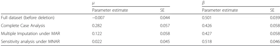
Complete case analysis and MI under MAR (withm= 300) were used for handling missing data and the weighting ap-proach was performed as a sensitivity analysis under MNAR following MI (setting δ= 0.2). Table 1 shows the empirical mean and standard deviation of the estimated pa-rameters of interest for the different methods of handling the missing data as well as for the full dataset before values ofYwere set to missing. According to the table, the esti-mated marginal mean ofY(μ) and the coefficientβ1from
the linear regression ofYon Xin the full dataset are very close to their true values (0 and 0.5, respectively). Under the complete case analysis, these estimates are far away from the full data values with large differences mainly in the estimate of the marginal mean as expected. The abso-lute difference of the MI estimates under MAR from the estimated values of the parameters of interest from the full dataset are 0.129 (i.e. 2.93 standard errors) and 0.074 (i.e.
Table 1Estimates of the marginal mean of the normally distributed outcome variable and the regression coefficient under four analysis methods for a single simulated dataset (n= 500, m =300,δ= 0.2)
μ β
Parameter estimate SE Parameter estimate SE
Full dataset (before deletion) −0.007 0.044 0.501 0.039
Complete Case Analysis 0.282 0.057 0.426 0.058
Multiple Imputation under MAR 0.122 0.058 0.427 0.058
1.89 standard errors), for the marginal mean ofYand the coefficientβ1, respectively. The estimate from the sensitivity
analysis under MNAR is 0.022 for the marginal mean and 0.518 for the measure of association, which are quite close to the values from the full dataset. This occurs as a result of using the true value ofδin the analysis; however, this can-not be expected in practice because the value of δ is unknown.
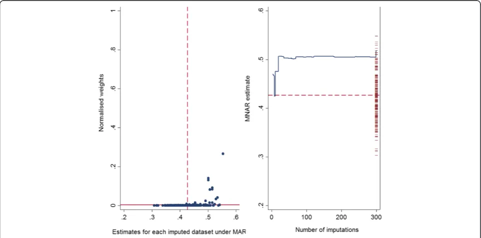
Graphical diagnostics explained earlier were applied in this single simulated dataset. As seen in Fig. 1, there is no extreme weight observed across the imputed datasets and the largest normalised weight is around 0.26 (left panel). In addition, the vertical drop observed in the running mean of the MNAR estimate at the early imputations ap-pears to settle down as the number of imputations in-creases and the estimate is not at the edge of the range of the 300 MAR estimates (right panel). See Additional file 3: Figure S3, for graphical diagnostics for the marginal mean of theYvariable; for this parameter the running mean of the MNAR estimate is at the edge of the MAR estimates.
Results of simulation experiment
The estimates of the marginal mean of the partially ob-served normally distributed outcome variable using complete case analysis, MI under MAR, and the sensitiv-ity analysis using the weighting approach under MNAR are shown in Table 2. The table presents the averaged estimates across the 1000 simulated datasets for the
different values ofm. Note that since the estimates based on the full dataset and complete case analysis do not de-pend on the number of imputations, their corresponding results are shown only in the first column of the Table (i.e.m= 5).
According to Table 2, estimates obtained from the complete case analysis and MI under MAR overestimate the true value, as expected. The MNAR estimates of the marginal mean using the weighting method reduce as the number of imputations increase, but importantly do
not converge to the value of the true mean as m
increases.
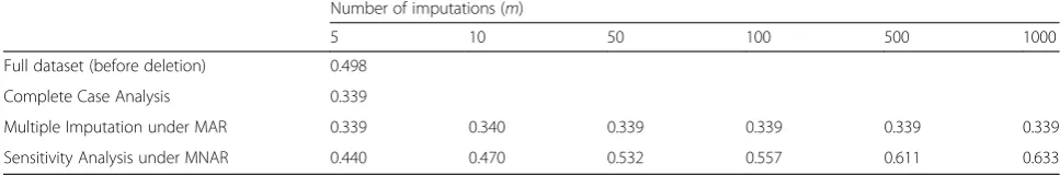
Table 3 presents estimates of the regression coefficient obtained using the four methods. As seen in the table, the mean estimate ofβ1across the 1000 simulated
data-sets for the full dataset is close to 0.5, as expected. The estimates for the complete case analysis and MI are similar and both are downwardly biased. The estimates under the MNAR sensitivity analysis increase with the number of imputations, and again do not converge to the true value ofβ1as m→∞. The results show that the
absolute bias in the sensitivity analysis reduces to 0.028 (or ~5 %) after 10 imputations, but then rises with the number of imputations to a value of 0.135 (or ~27 %) for 1000 imputations.
Further examination was carried out for estimating the marginal mean of the partially observed normally dis-tributed outcome variable and the regression coefficient
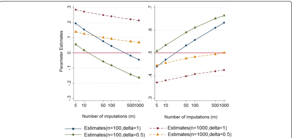
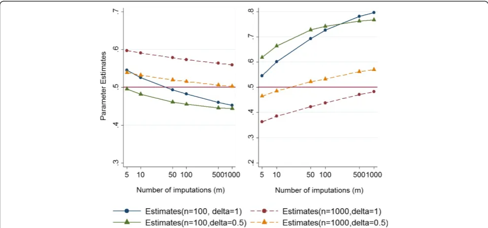
by 1) increasing the sample size of the simulated data-sets from 100 to 1000; and 2) reducing the magnitude of departure from the MAR assumption (δ) from 1 to 0.5. A summary of the results for different scenarios is pre-sented in the following graphs. According to the results presented in Fig. 2:
i. The parameter estimates decrease for the marginal mean and increase for the regression coefficient
^
β1 as the number of imputations increases. The
estimates appear to be converging to a single biased estimate (on the original scale); except potentially for the scenario with a large sample size (n= 1000) and a moderate departure from MAR (δ= 0.5). However, based on the observed patterns, it seems that by applying more imputations, the estimates obtained from a largenand moderateδwill move further away from the true value ifmexceeds 1000. ii. Surprisingly, the parameter estimates are lower for
the marginal mean (left panel) and higher for the measure of association (right panel) forδ= 0.5 compared withδ= 1. It seems that we are observing two opposing effects here. One possible explanation for this observation might be the fact that while increasingδfrom 0.5 to 1 in the MNAR analysis increases the potential for extreme weights, increasingδin the data generating mechanism reduces the left-hand tail of the observed outcome distribution and thus, reduces the potential for extreme weights.
Further investigation
We extended our simulation study to account for a par-tially observed binary outcome variable and a fully ob-served continuous covariate. The estimates of the marginal proportion of the binary outcome and the re-gression coefficient obtained from complete case ana-lysis, MI under MAR, and the sensitivity analysis using the weighting approach under MNAR are summarised in Tables 4 and 5, respectively. It is apparent from Tables 4 and 5 that the results of the complete case ana-lysis and MI under MAR are biased, as expected. Again the MNAR estimates decrease for estimating the mar-ginal proportion of the outcome variable as the number of imputations increase and do not converge towards the true value of the parameter (Table 4). Also, the esti-mates from the sensitivity analysis for the regression
co-efficient increase as the number of imputations
increases, thus moving further away from the true value (Table 5).
Additional examination was carried out when the sam-ple size of the simulated data was increased from 100 to 1000 and the degree of departure from MAR reduced from 1 to 0.5. Again the results show biased estimates using complete case analysis and MI under MAR for both the marginal proportion of the partially observed outcome and the measure of association. Figure 3 pre-sents the parameter estimates of interest under MNAR (left panel: marginal proportion of the outcome variable and right panel: exposure-outcome relationship) against the number of imputations, when the sample sizes are
Table 2Estimates of the marginal mean of the normally distributed outcome variable under four analysis methods (n= 100,δ= 1); True value = 0
Number of imputations (m)
5 10 50 100 500 1000
Full dataset (before deletion) −0.003
Complete Case Analysis 0.489
Multiple Imputation under MAR 0.323 0.322 0.322 0.322 0.322 0.322
Sensitivity Analysis under MNAR 0.196 0.155 0.078 0.046 −0.018 −0.044
Note:The empirical Monte Carlo standard errors were all around 0.003 for MI and 0.004 for sensitivity analysis
Table 3Estimates of the linear regression coefficient (β1) under four analysis methods (n = 100,δ= 1); True value = 0.5
Number of imputations (m)
5 10 50 100 500 1000
Full dataset (before deletion) 0.498
Complete Case Analysis 0.339
Multiple Imputation under MAR 0.339 0.340 0.339 0.339 0.339 0.339
Sensitivity Analysis under MNAR 0.440 0.470 0.532 0.557 0.611 0.633
100 and 1000 andδare 1 and 0.5. The Figure illustrates almost the same pattern as Fig. 2; that is, the MNAR es-timates do not approach the true parameter values as
m→∞.
Explanation of the method failure
In this section, we discuss further details of the weight-ing approach within the MI framework, which may ex-plain why the weighting approach fails, as observed in the previous section.
Consider imputation in the setting described under the first model in the“Methods”section (i.e. normally distrib-uted outcome (partially observed) and covariate (fully ob-served)). Initially, the linear regression model, Y=β0
+β1X+ε; (ε∼N(0,σ2)), is fitted to the observed data in order to obtain the point estimates ofβ^ (i.e.β^0 Andβ^1in this example) and σ^2. Then, a new parameter estimateβ*
and its associated variance (σ*2) are drawn from their joint
posterior distribution in two steps:
σ2∼σ^2ðno−qÞ χ2
no−q
ð12Þ
β σ2∼N β^;σ2 X′oXo
−1
ð13Þ
wheren0denotes the number of complete cases (i.e. ob-served data values for Yin this example),q is the num-ber of parameters in the linear regression model (i.e. two for this simulation example) and Xo corresponds to the
X values where the Y values are also observed (i.e. the complete cases) [6].
One reason why the weighting approach may fail is be-cause the posterior predictive distribution of Ygiven X, from which the imputations for this example are drawn, is a Student-t distribution. This is because the imputation
Fig. 2Estimates of the marginal mean (left panel) and the regression coefficient (right panel) for a normally distributed outcome obtained from the sensitivity analysis under MNAR against number of imputations (m) on a log scale
Table 4Estimates of the marginal proportion of the binary outcome variable under four analysis methods (n= 100,δ= 1); True value = 0.5
Number of imputations (m)
5 10 50 100 500 1000
Full dataset (before deletion) 0.497
Complete Case Analysis 0.639
Multiple Imputation under MAR 0.608 0.608 0.608 0.608 0.608 0.608
Sensitivity Analysis under MNAR 0.545 0.526 0.493 0.482 0.460 0.452
parameterσ*2follows a scaled inverse chi-squared
distribu-tion, shown in Equation (12), and the true variance is un-known. Importantly, the tails of the probability density function of the t-distribution follow a power function. Against that, the weights have the form of an exponential function (refer to Equation (6)); thus, in the tail of the dis-tribution of the imputed values Σi∈IYYij, the weights
in-crease more quickly than the density of the distribution decreases. It can be shown that, across the imputed data-sets and given the observed data, the sum of Yi in Equation (6) (i.e.Σi∈IYYij, whereiindicates thei
th
imputed value and jrepresents jth imputed dataset) itself has a t -distribution withn0-qdegrees of freedom, wheren0is the number of observed values. This links more closely the shape of the imputation distribution to the shape of the weight function. Consequently, the second condition of the importance sampling is violated as the weight, the ra-tio of the imputara-tion distribura-tion under MNAR to the im-putation distribution under MAR (g/f described in the
“Importance sampling” section), is unbounded. This re-sults in an inconsistent MNAR estimate, and may explain why the weighting approach fails in our example.
Note that the explanation above does not apply to a binary outcome variable, since the imputation distribu-tion is no longer a t-distribution. In fact, β* is drawn
from the asymptotic approximation to its posterior dis-tribution, and the imputed values are only approximate draws from the posterior predictive distribution of the missing data. However, in many cases, this asymptotic approximation may not be an accurate approximation to the joint posterior distribution, as it might be extremely wrong out in the tails of the distribution. Thus, again in the context of an incomplete binary variable it appears that the importance weights become unbounded and the MNAR estimate may remain unstable.
It is worth mentioning that thet-distribution is similar to the normal distribution, but with heavier tails for small sample sizes. As the sample size increases, the
Table 5Estimates of the logistic regression coefficient (φ1) under four analysis methods (n= 100,δ= 1); True value = 0.5
Number of imputations (m)
5 10 50 100 500 1000
Full dataset (before deletion) 0.524
Complete Case Analysis 0.329
Multiple Imputation under MAR 0.331 0.332 0.331 0.331 0.332 0.332
Sensitivity Analysis under MNAR 0.546 0.601 0.693 0.727 0.781 0.797
Note: The empirical Monte Carlo standard errors were all around 0.008 for MI for sensitivity analysis
degrees of freedom (df) increases and the t-distribution approaches the normal distribution. For datasets that are small or the number of missing values is large, the miss-ing observations are drawn from a t-distribution with heavy tails. As a result, the MNAR estimate becomes even more unstable in these scenarios since, across im-puted datasets, the MAR estimate may become noisier and improperly weighted. Of note, the problem of un-bounded weights is not restricted to small sample sizes; but it becomes more evident when the sample size is small since the imputed values are drawn from much heavier tails of the posterior predictive distribution of missing data. Hence, this issue extends to all datasets ir-respective of sample size.
In general, it seems that as we increase the number of imputations, the more likely we are to draw a really ex-treme imputed dataset which is assigned nearly all the weight. The problem arises because the weight used for calculating the overall MNAR estimate is not actually the ratio of t-densities, and thus, the ratio is definitely unbounded unless the Yi’s are bounded. In fact, this problem occurs as a result of a failure in the argument of Carpenter et al. [18]. In their paper it was shown that the importance ratio, which was described in the “ Im-portance sampling”section, is
g f ¼
f½Y Xj ;R¼0 f½Y Xj ;R¼1
¼f½R¼0jY;X
f½R¼1jY;X
f X½ ;R¼1 f X½ ;R¼0 ð14Þ
where, in a simple scenario, there was only one individ-ual with a fully observed covariateX, a partially observed response Y, and a missingness indicator R, which was zero ifYwas missing. It was claimed that under the lo-gistic model in Equation (3), f[R= 1|Y,X] equates to expit(α+γX+δY), and thus the importance ratio was simplified as expf−½αþγXþδYgff½½XX;;RR¼¼10∝expð−δYÞ. However, this simplification relies on the assumption that all the parameters are known. A correct weighting would computef[R=r|Y,X], where r = 0,1 by integrating
f[R=r|Y,X,α,γ,δ] over the posterior distribution of α and γ in the numerator and denominator in Equation (14).
In the more general case of imputation models that are GLMs (e.g. logistic regression), where the imputation models make a normal approximation to the posterior, it seems that the weighting method will also fail because of the reason mentioned above. However, this could poten-tially be avoided for binary variables with missing data by applying bootstrapping in the imputation process. The idea is to draw a single bootstrap sample (i.e. ran-dom sampling with replacement) from the data (multiple times) and fitting the imputation model to the bootstrap
sample in order to avoid situations where the asymptotic approximation may be inadequate for the posterior dis-tribution [44].
It seems that the method failure is likely to occur more obviously in smaller samples, since they have smaller degrees of freedom. Also, the bias in the MNAR estimate will probably increase as the number of imputa-tions increases in smaller datasets. Furthermore, the lar-gest weight will increase as the number of imputations increases and the MNAR estimate will become unstable (because the chance of observing an imputed dataset with the minimal sum of the imputed values (for δ> 0), or with a maximal sum of imputed values (forδ< 0) in-creases asmincreases).
Graphical method for selectingδ
In the simulation studies described earlier, we considered an unrealistic situation where we assumed that the value of δwas known. In this section, we describe a real situ-ation where the value ofδis unknown, and then apply the graphical method proposed by Héraud-Bousquet et al. [30] to select a range of plausible values forδ.
Overview of procedure for choosingδ
In the absence of sufficient information about the un-measured factors in a dataset, it is not typically possible to estimate the degree of departures from the MAR mechanism for performing a sensitivity analysis in practice.
One way to select the magnitude of departures from MAR is to elicit all possible values that would be consid-ered reasonable by experts. Héraud-Bousquet et al. [30] have recently developed a graphical method for obtain-ing a range of plausible values ofδwhich represent local departures from the MAR assumption. This graphical method was illustrated in four steps using epidemio-logical data from an observational cohort, in which nor-malised weights for each imputed dataset were plotted against different possible values ofδ.
According to Héraud-Bousquet et al.’s suggestion for obtaining a range ofδ, the maximum normalised weight should be around 0.5, and at least five normalised weights should be above 1
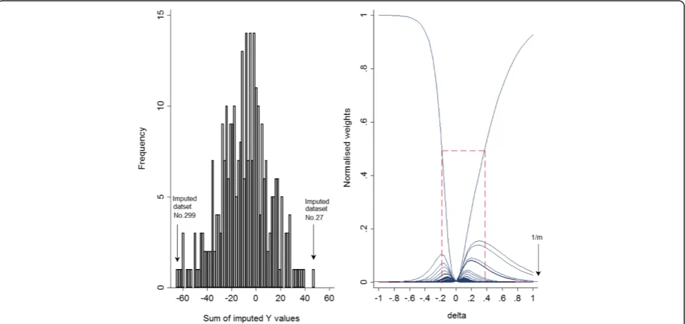
Illustration using a single simulated dataset(continued) We first start with the single simulated data example de-scribed earlier and apply the graphical method for choosing a range forδ, and then we extend our example to larger magnitudes ofδ. Figure 4 shows a histogram of the sum of imputed Y values in each of 300 imputed datasets (left panel) and the normalised weights based on different δ values (right panel), where each curve is plotted as a function of δ, with a different function for each of the 300 imputed datasets.
Héraud-Bousquet et al. [30] mentioned that the max-imum normalised weight across the imputed datasets cor-responds to the imputed dataset with the minimum sum of the imputed values when δ is positive (δ> 0), or the maximum sum of the imputed values when δis negative (δ< 0). As can be seen, the datasets no. 299 and 27 have the minimum and maximum sum of imputations, respect-ively (refer to the left panel of Fig. 4). Since the true value ofδis 0.2 in this dataset, the maximum normalised weight corresponds to the dataset no. 299 since this has the mini-mum sum of imputed values.
The right panel of Fig. 4 presents the normalised weights against different δ values. According to Hér-aud-Bousquet, et al., the maximum normalised weight should be around 0.5, and more than 5 normalised weights should be above the line of 3001 . The range of
δ values that fit these criteria is shown by dashed lines. This range includes values of δ between −0.18
and 0.38 and captures the true value of δ (0.2) used to simulate the data.
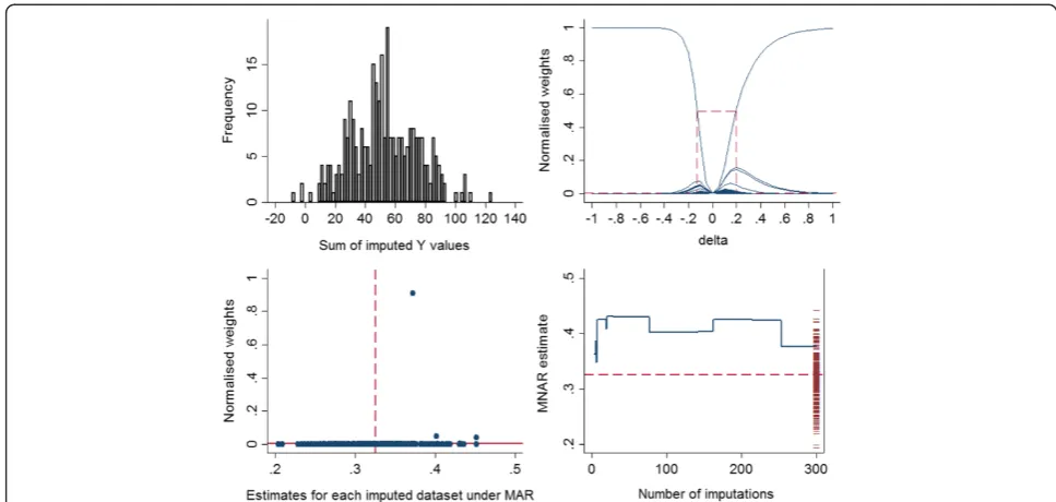
Further investigation was carried out by increasing the magnitude of δ in the simulated data to 0.5 and 1, with everything else identical. Figure 5 shows the graphical procedure for selecting a range forδand graphical diag-nostics explained in the section “Graphical diagnostics”, for the measure of association when n= 500, m= 300 and the trueδis 1.
It is apparent that the range for δ obtained from the plot above (−0.13, 0.2) does not capture the true value of
δ =1 for this dataset (top right panel). There is a single imputed dataset which has a high weight, meaning that this imputed dataset is very influential. Further examin-ation showed that about 99 % of the weight was concen-trated on this single imputed dataset, which corresponds to the outlying weight in the bottom left panel of Fig. 5, and the large vertical drop at 253 imputed datasets in the bottom right panel of Fig. 5. See Additional file 4: Table S1 for estimates of the parameters of interest, with 95 % CI and SE, and Additional file 5: Figure S4, for the graphical diagnostics for the marginal mean of the Y
variable.
The same results were observed when the moderate magnitude of departure from MAR was selected (δ= 0.5) (see Additional file 6: Table S2, Additional file 7: Figure S5 and Additional file 8: Figure S6). Surprisingly, even when the sample size was increased from 500 to
1000, with a small value of departure δ= 0.2 one im-puted dataset was again given a very large weight (see Additional file 9: Table S3, Additional file 10: Figure S7 and Additional file 11: Figure S8).
Discussion
MI is a common approach for handling missing data. Standard implementation of MI assumes the data are MAR, so it is widely recommended to perform a sensi-tivity analysis to explore the robustness of inferences to departures from the MAR assumption.
This study evaluated a selection-model-based weighting approach for performing a sensitivity analysis within the MI framework. Simulation studies were designed to assess whether the proposed method can provide unbiased MNAR estimates across varying numbers of imputations and sample sizes where the magnitude of departures from MAR varied from moderate to large. The results indicate that, in general, the weighting approach produces highly unstable MNAR estimates across varying numbers of im-putations. This study also evaluated the graphical method proposed by Héraud-Bousquet et al. [30] for obtaining a range of plausible values of the sensitivity parameterδ(i.e. the magnitude of departure from the MAR assumption) to examine whether the plausible value is far away from the true value.
Carpenter et al. [18] introduced the weighting ap-proach and showed that, in a single simulation study, this method can gradually remove the bias in the MNAR
estimate as the number of imputations increases. Fur-ther, Carpenter and Kenward [6] noted that if the dataset is small or contains a large number of missing values, by increasing the number of imputations the MNAR esti-mate obtained from the weighting approach might be unstable; however, if a suitable imputation model is chosen the method will perform well in small datasets. A partial solution has been recently developed when performing the weighting approach in small datasets (personal communication: James Carpenter and Melanie Smuk).
In a different application of the weighting approach where MI followed by re-weighting was used to assess the sensitivity of the pooled estimate in a meta-analysis to selection bias, Carpenter et al. [45] commented on how the importance ratio will become unbounded as se-lection bias of studies included in the meta-analysis in-creases. In their paper they proposed a correction to the weights formula and illustrated that this performed well when there was a moderate selection bias and more than 10 observed studies included in the meta-analysis.
The simulation study that was carried out by Carpenter et al. [18] was the same as our study described in the
“Methods” section (n= 100, δ= 1) where the marginal mean of a partially observed continuous outcome variable was the parameter of interest. We extended their simula-tion study to investigate the addisimula-tional parameter, the re-gression coefficient for the outcome on the exposure variable. In our simulation studies, we identified that
Fig. 5Graphical procedure for selecting a range forδ(top). Top left panel: histogram of the sum of imputedYvalues for each dataset. Top right panel: graphical determination of delta for the variableYusing the approach suggested by Héraud-Bousquet et al. [30]. Graphical
the MNAR estimates were biased and did not con-verge to the true value of the parameters of interest for either the marginal mean of the outcome or the regression coefficient as the number of imputations increased. A similar pattern was also apparent in the simulation study by Carpenter et al. [18], where at 1000 imputations the MNAR estimate was negative (−0.01), and based on our findings, we expect this es-timate would move further away from zero if more than 1000 imputations were performed. Of note, there is a small discrepancy observed between our MNAR estimates and the original article by Carpenter et al. [18], over increasing number of imputations (≥50 im-putations). One explanation for these discrepancies is stochastic variability in the imputation process that increases with the number of imputations. That is, the random draws of the imputation model parame-ters from their posterior distributions for creating the imputed values. In particular, increasing the number of imputations increases the chance of drawing an ex-treme imputed dataset that is assigned an exex-treme weight. Consequently, the MNAR estimate becomes highly dependent on that single imputed dataset as the number of imputations increases, and thus the distribution of the MNAR estimates over 1000 impu-tations has wider tails than the distribution over fewer imputations. Our investigation shows that the distribution of simulated point estimates is heavy-tailed in such a way that Normal-theory confidence intervals fail. Therefore, in such cases, Monte Carlo errors may be a poor guide to simulation error.
Biased estimates were also observed when we in-creased the sample size to 1000, explored a moderate departure in the MAR assumption (δ= 0.5), and ex-tended our evaluation to a binary (partially observed) outcome variable.
The findings of our investigation highlight that the weights used in estimating the overall parameter esti-mate under MNAR become unbounded as the number of imputations increases. This leads to improper weight-ing of the imputed datasets so that one or two datasets take approximately all the weight. It was shown that the problem of large weights occurs not only for large de-parture from MAR, but it also may occur for small and moderate departures even in large datasets. As explained in the section “Explanation of the method failure”, the problem arises from the computation of the weights, and this method should work better if the weights were correctly computed. However, this issue may not have a simple solution that is computationally convenient.
The graphical method proposed by Héraud-Bousquet, et al. [30] for selecting δ relies heavily on the (normal-ised) weights, which themselves depend on the imputed values under MAR. This limits the usefulness of this
approach. By definition, we cannot estimate δ from the data at hand; hence, obtaining a range for δ based on the available data seems inherently implausible. In fact, our findings demonstrate that this method does not per-form adequately as a graphical approach for selecting a range of δ did not capture the true value of δ used in our simulation studies. Unfortunately, satisfactory guide-lines are not currently available in the literature regard-ing the selection of δfor performing sensitivity analyses via MI, and further research is required to develop strat-egies if this is going to be a worthwhile avenue to
pur-sue. The only principled approach to determine
clinically plausible values of δ is to elicit these from pert knowledge informed as much as possible from ex-ternal empirical evidence [35, 37]. This approach has been adopted in other areas of statistics [46, 47].
An alternative approach to assess the impact of de-parture from the MAR assumption within the MI frame-work is the pattern-mixture approach [6, 20, 21, 35]. This method is straightforward and easier to compre-hend for non-statistical collaborators compared with the weighting approach [29]. Under the pattern-mixture ap-proach, the degree of departure from MAR is defined as the difference (shift) in the mean of a partially observed variable between the unobserved and observed data. Within the MI framework, this alternative approach is applicable for both partially observed outcomes and co-variates, and potentially when more than one variable has missing data. In the case of a continuous partially observed variable, missing data are imputed using stand-ard MI assuming MAR, and then the imputed values in each imputed datasets are shifted (i.e. add or multiply
δpm, a pattern-mixture model sensitivity parameter, to
each of the imputed values) in such a way that they rep-resent the MNAR mechanism. When there is a partially observed binary variable, the shift of δpm needs to be
added to the imputation model; therefore the missing values are, in fact, drawn from an imputation model as-suming MNAR rather than MAR. More technical details of this approach are provided by Carpenter and Kenward [6], Ratitch et al. [20], Siddique et al. [48, 49], and White et al. [35].
Conclusions
potential for bias using the weights proposed by Carpenter et al. should be recognised by users, and more appropriate methods should be developed. Hence, add-itional investigation into MNAR approaches perhaps with more focus on the pattern-mixture approach as an alternative method for conducting a sensitivity analysis following MI is desirable.
Additional files
Additional file 1: Figure S1.Procedure for performing a simulation study for a normally distributed outcome. (DOCX 31 kb)
Additional file 2: Figure S2.Procedure for performing a simulation study for a binary outcome variable. (DOCX 31 kb)
Additional file 3: Figure S3.Graphical diagnostics for a single simulated dataset (n= 500,m= 300,δ(True)= 0.2,μ(True)= 0,μðSimulateÞ=−0.007).
(DOCX 2362 kb)
Additional file 4: Table S1.Estimates of the marginal mean of the normally distributed outcome variable and the regression coefficient under four analysis methods for a single simulated dataset (n= 500, m =300,δ= 1). (DOCX 18 kb)
Additional file 5: Figure S4.Graphical diagnostics for a single simulated dataset (n= 500,m= 300,δ(True)= 1,μ(True)= 0,^μðSimulateÞ=−0.007).
(DOCX 2362 kb)
Additional file 6: Table S2.Estimates of the marginal mean of the normally distributed outcome variable and the regression coefficient under four analysis methods for a single simulated dataset (n= 500, m =300,δ= 0.5). (DOCX 17 kb)
Additional file 7: Figure S5.Graphical procedure for selecting a range forδ(top). Top left panel: histogram of the sum of imputedYvalues for each data set. Top right panel: graphical determination of delta for the variableYusing the approach suggested by Héraud-Bousquet et al. Graphical diagnostics (bottom). Bottom left panel: normalised weights against the MAR estimates obtained from each of the 500 imputed dataset. Bottom right panel: mean of the MNAR estimate against the number of imputations (n= 500,m= 300,δ(True)= 0.5,β(True)= 0.5, βðSimulateÞ=0.501). (DOCX 2362 kb)
Additional file 8: Figure S6.Graphical diagnostics for a single simulated dataset (n= 500,m= 300,δ(True)=0.5,μ(True)=0,μ^ðSimulateÞ=−0.007). (DOCX
2362 kb)
Additional file 9: Table S3.Estimates of the marginal mean of the normally distributed outcome variable and the regression coefficient under four analysis methods for a single simulated dataset(n= 1000, m =500,δ= 0.2). (DOCX 17 kb)
Additional file 10: Figure S7.Graphical procedure for selecting a range forδ(top). Top left panel: histogram of the sum of imputedYvalues for each data set. Top right panel: graphical determination of delta for the variableYusing the approach suggested by Héraud-Bousquet et al. Graphical diagnostics (bottom). Bottom left panel: normalised weights against the MAR estimates obtained from each of the 500 imputed dataset. Bottom right panel: mean of the MNAR estimate against the number of imputations (n= 1000,m= 500,δ(True)= 0.2,β(True)= 0.5,β^ðSimulateÞ=0.498).
(DOCX 2362 kb)
Additional file 11: Figure S8.Graphical diagnostics for a single simulated dataset (n= 1000,m= 500,δ(True)= 0.2,μ(True)= 0,μðSimulateÞ=−0.009).
(DOCX 2362 kb)
Abbreviations
CC:Complete case; DF: Degrees of freedom; MAR: Missing at random; MCAR: Missing completely at random; MI: Multiple imputation; MNAR: Missing not at random; SE: Standard Error.
Competing interest
The authors declare that they have no competing interests.
Authors’contributions
PHR designed the simulation study, performed the analysis, and drafted the manuscript. JAS conceived of the idea for the simulation study, participated in designing the simulation study and helped in writing of the manuscript. IRW provided theoretical input and revised the manuscript. KJL and JBC contributed to the design of the simulation study and revised the manuscript. All authors contributed to the interpretation of the results, and read and approved the final manuscript.
Authors’information
Not applicable.
Availability of data and materials Not applicable.
Acknowledgements
This work was supported by funding from the National Health and Medical Research Council: a Centre of Research Excellence grant, ID 1035261, awarded to the Victorian Centre of Biostatistics (ViCBiostat), and Career Development Fellowship ID 1053609(KJL). PHR is funded by an Australian Postgraduate Award. IRW was supported by the Medical Research Council [Unit Programme number U105260558].
Author details
1Centre for Epidemiology and Biostatistics, Melbourne School of Population
and Global Health, The University of Melbourne, Parkville, Melbourne, VIC, Australia.2MRC Biostatistics Unit, Cambridge Institute of Public Health, Cambridge CB2 0SR, UK.3Clinical Epidemiology and Biostatistics Unit, Murdoch Childrens Research Institute, Parkville, Melbourne, VIC, Australia. 4Department of Paediatrics, The University of Melbourne, Parkville,
Melbourne, VIC, Australia.
Received: 3 June 2015 Accepted: 28 September 2015
References
1. Hayati Rezvan P, Lee KJ, Simpson JA. The rise of multiple imputation: a review of the reporting and implementation of the method in medical research. BMC Med Res Methodol. 2015;15(1):1–14.
2. Bell ML, Fiero M, Horton NJ, Chiu-Hsieh H. Handling missing data in RCTs; a review of the top medical journals. BMC Med Res Methodol. 2014;14(1):1–16. 3. Powney M, Williamson P, Kirkham J, Kolamunnage-Dona R. A review of the
handling of missing longitudinal outcome data in clinical trials. Trials. 2014;15(1):1–19.
4. Karahalios A, Baglietto L, Carlin JB, English DR, Simpson JA. A review of the reporting and handling of missing data in cohort studies with repeated assessment of exposure measures. BMC Med Res Methodol. 2012;12:96–105. 5. Wood AM, White IR, Thompson SG. Are missing outcome data adequately
handled? A review of published randomized controlled trials in major medical journals. Clin Trials. 2004;1(4):368–76.
6. Carpenter JR, Kenward MG. Multiple imputation and its application/James R. Carpenter and Michael G. Kenward. 1st ed. Chichester: Wiley; 2013. 7. Little RJA, Rubin DB. Statistical analysis with missing data/Roderick J.A. Little,
Donald B. Rubin. 2nd ed. Hoboken: Wiley; 2002.
8. Schafer JL, Graham JW. Missing data: Our view of the state of the art. Psychol Methods. 2002;7(2):147–77.
9. R Development Core Team. R: A language and environment for statistical computing, reference index version 2.2.1. Vienna, Austria. ISBN 3-900051-07-0. URL http://www.R-project.org.: R Foundation for Statistical Computing; 2005.
10. SAS Institute Inc. PROC MI. SAS Procedures Giude, Version 9.2. Cary: SAS Institute Inc; 2008.
11. StataCorp. Stata Statistical Software: Release 12. College Station, TX. College Station, TX: Stata Corp LP; 2009.
12. Mackinnon A. The use and reporting of multiple imputation in medical research - a review. J Intern Med. 2010;268(6):586–93.
13. Sterne JAC, White IR, Carlin JB, Spratt M, Royston P, Kenward MG, et al. Multiple imputation for missing data in epidemiological and clinical research: Potential and pitfalls. BMJ (Online). 2009;339(7713):157–60. 14. Kenward MG, Carpenter J. Multiple imputation: current perspectives. Stat
15. Rubin DB. Multiple imputation for nonresponse in surveys/Donald B. Rubin. New York: Wiley; 1987.
16. Schafer JL. Analysis of incomplete multivariate data. 1st ed. Boca Raton: Chapman & Hall/CRC; 1997.
17. White IR, Carlin JB. Bias and efficiency of multiple imputation compared with complete-case analysis for missing covariate values. Stat Med. 2010;29(28):2920–31.
18. Carpenter JR, Kenward MG, White IR. Sensitivity analysis after multiple imputation under missing at random: a weighting approach. Stat Methods Med Res. 2007;16(3):259–75.
19. O'Kelly M, Ratitch B. Clinical trials with missing data : a guide for practitioners / Michael O’Kelly, Bohdana Ratitch. Chichester: John Wiley & Sons; 2014.
20. Ratitch B, O'Kelly M, Tosiello R. Missing data in clinical trials: from clinical assumptions to statistical analysis using pattern mixture models. Pharm Stat. 2013;12(6):337–47.
21. van Buuren S, Boshuizen HC, Knook DL. Multiple imputation of missing blood pressure covariates in survival analysis. Stat Med. 1999;18(6):681–94. 22. Kenward M, Molenberghs G. Parametric models for incomplete continuous
and categorical longitudinal data. Stat Methods Med Res. 1999;8(1):51–83. 23. Hogan JW, Laird NM. Model-Based Approaches To Analysing Incomplete
Longitudinal And Failure Time Data. Stat Med. 1997;16(3):259–72. 24. Little RJA. Modeling the drop-out mechanism in repeated-measures studies.
J Am Stat Assoc. 1995;90(431):1112–21.
25. Diggle P, Kenward MG. Informative Drop-out in Longitudinal Data Analysis. J R Stat Soc: Ser C: Appl Stat. 1994;43(1):49–93.
26. Little RJA. Pattern-Mixture Models for Multivariate Incomplete Data. J Am Stat Assoc. 1993;88(421):125–34.
27. Yuan Y. Sensitivity Analysis in Multiple Imputation for Missing Data. In Proceedings of the SAS Global Forum 2014 Conference:[http:// support.sas.com/resources/papers/proceedings14/SAS270-2014.pdf]. 28. Resseguier N, Giorgi R, Paoletti X. Sensitivity analysis when data are missing
not-at-random. Epidemiology. 2011;22(2):282–3.
29. Daniels MJ, Hogan JW. Missing data in longitudinal studies : strategies for Bayesian modeling and sensitivity analysis / Michael J. Daniels, Joseph W. Hogan. Boca Raton: Chapman & Hall/CRC; 2008.
30. Héraud-Bousquet V, Larsen C, Carpenter J, Desenclos J, Le Strat Y. Practical considerations for sensitivity analysis after multiple imputation applied to epidemiological studies with incomplete data. BMC Med Res Methodol. 2012;12:73–83.
31. Rasbah J. A user’s guide to MLwiN, version 2.10: Centre for Multilevel Modelling. Bristol, UK: University of Bristol; 2009.
32. Gilks WR, Richardson S, Spiegelhalter DJ. Markov chain Monte Carlo in practice. London; Melbourne: Chapman & Hall; 1996.
33. Molenberghs G, Beunkens C, Jansen I, Thijs H, van Steen K, Verbeke G, et al. Analysis of incomplete data. In: Dmitrienko A, Chuang-Stein C, D'Agostino RB, editors. Pharmaceutical statistics using SAS : a practical guide. Cary, NC: SAS publishing; 2007. p. 313.
34. Kenward MG. Selection models for repeated measurements with non-random dropout: an illustration of sensitivity. Stat Med. 1998;17(23):2723–32. 35. White IR, Carpenter J, Evans S, Schroter S. Eliciting and using expert
opinions about dropout bias in randomized controlled trials. Clin Trials. 2007;4(2):125–39.
36. O'Hagan A. Eliciting Expert Beliefs in Substantial Practical Applications. J R Stat Soc Series D. 1998;47(1):21–35.
37. Kadane JB, Wolfson LJ. Experiences in Elicitation. J R Stat Soc Series D. 1998;47(1):3–19.
38. Gelman A, Carlin JB, Stern HS, Dunson DB, Vehtari A, Rubin DB. Bayesian data analysis. 3rd ed. Boca Raton: CRC Press; 2014.
39. Hesterberg T. Weighted average importance sampling and defensive mixture distributions. Technometrics. 1995;37(2):185–94.
40. Agresti A. An introduction to categorical data analysis/Alan Agresti. 2nd ed. Hoboken, NJ: Wiley-Interscience; 2007.
41. van Buuren S. Flexible Imputation of Missing Data. 1st ed. Hoboken: Taylor and Francis; 2012.
42. White IR, Royston P, Wood AM. Multiple imputation using chained equations: Issues and guidance for practice. Stat Med. 2011;30(4):377–99. 43. Royston P. Multiple imputation of missing values. STATA J. 2004;4(3):227–41. 44. White IR, Daniel R, Royston P. Avoiding bias due to perfect prediction in
multiple imputation of incomplete categorical variables. Comput Stat Data Anal. 2010;54:2267–75.
45. Carpenter J, Rücker G, Schwarzer G. Assessing the Sensitivity of Meta-analysis to Selection Bias: A Multiple Imputation Approach. Biometrics. 2011;67(3):1066–72.
46. Bond SJ, White IR. Estimating causal effects using prior information on nontrial treatments. Clin Trials. 2010;7(6):664–76.
47. Turner RM, Spiegelhalter DJ, Smith GCS, Thompson SG. Bias modelling in evidence synthesis. J R Stat Soc Series A. 2009;172(1):21–47.
48. Siddique J, Harel O, Crespi CM. Addressing Missing Data Mechanism Uncertainty using Multiple-Model Multiple Imputation: Application to a Longitudinal Clinical Trial. Ann Appl Stat. 2012;6(4):1814–37.
49. Siddique J, Harel O, Crespi CM, Hedeker D. Binary variable multiple-model multiple imputation to address missing data mechanism uncertainty: application to a smoking cessation trial. Stat Med. 2014;33(17):3013–28.
Submit your next manuscript to BioMed Central and take full advantage of:
• Convenient online submission
• Thorough peer review
• No space constraints or color figure charges
• Immediate publication on acceptance
• Inclusion in PubMed, CAS, Scopus and Google Scholar
• Research which is freely available for redistribution