R E G U L A R A R T I C L E
Heat-related mortality risk model for climate
change impact projection
Yasushi Honda•Masahide Kondo •Glenn McGregor•Ho Kim • Yue-Leon Guo•Yasuaki Hijioka•Minoru Yoshikawa•Kazutaka Oka• Saneyuki Takano• Simon Hales•R. Sari Kovats
Received: 31 January 2013 / Accepted: 11 July 2013 / Published online: 9 August 2013 ÓThe Japanese Society for Hygiene 2013
Abstract
Objectives We previously developed a model for pro-jection of heat-related mortality attributable to climate change. The objective of this paper is to improve the fit and precision of and examine the robustness of the model.
Methods We obtained daily data for number of deaths and maximum temperature from respective governmental organizations of Japan, Korea, Taiwan, the USA, and European countries. For future projection, we used the Bergen climate model 2 (BCM2) general circulation model, the Special Report on Emissions Scenarios (SRES) A1B socioeconomic scenario, and the mortality projection for the 65?-year-old age group developed by the World Health Organization (WHO). The heat-related excess mortality was defined as follows: The temperature–mor-tality relation forms a V-shaped curve, and the temperature
at which mortality becomes lowest is called the optimum temperature (OT). The difference in mortality between the OT and a temperature beyond the OT is the excess mor-tality. To develop the model for projection, we used Jap-anese 47-prefecture data from 1972 to 2008. Using a distributed lag nonlinear model (two-dimensional non-parametric regression of temperature and its lag effect), we included the lag effect of temperature up to 15 days, and created a risk function curve on which the projection is based. As an example, we perform a future projection using the above-mentioned risk function. In the projection, we used 1961–1990 temperature as the baseline, and temper-atures in the 2030s and 2050s were projected using the BCM2 global circulation model, SRES A1B scenario, and WHO-provided annual mortality. Here, we used the ‘‘counterfactual method’’ to evaluate the climate change
Y. Honda (&)
Faculty of Health and Sport Sciences, University of Tsukuba, Comprehensive Research Building D 709, 1-1-1 Tennoudai, Tsukuba 305-8577, Japan
e-mail: honda@taiiku.tsukuba.ac.jp
M. Kondo
Faculty of Medicine, University of Tsukuba, Tsukuba, Japan
G. McGregor
School of Environment, University of Auckland, Greater Auckland, New Zealand
H. Kim
School of Public Health, Seoul National University, Seoul, South Korea
Y.-L. Guo
Environmental and Occupational Medicine, National Taiwan University (NTU) College of Medicine and NTU Hospital, Taipei, Republic of China
Y.-L. Guo
Institute of Occupational Medicine and Industrial Hygiene, National Taiwan University, Taipei, Republic of China
Y. Hijioka
Center for Social and Environmental Systems Research, National Institute for Environmental Studies, Tsukuba, Japan
M. YoshikawaK. OkaS. Takano
Environment and Energy Division 1, Mizuho Information and Research Institute, Tokyo, Japan
S. Hales
Department of Public Health, University of Otago, Dunedin, New Zealand
R. S. Kovats
impact; For example, baseline temperature and 2030 mortality were used to determine the baseline excess, and compared with the 2030 excess, for which we used 2030 temperature and 2030 mortality. In terms of adaptation to warmer climate, we assumed 0 % adaptation when the OT as of the current climate is used and 100 % adaptation when the OT as of the future climate is used. The midpoint of the OTs of the two types of adaptation was set to be the OT for 50 % adaptation.
Results We calculated heat-related excess mortality for 2030 and 2050.
Conclusions Our new model is considered to be better fit, and more precise and robust compared with the previous model.
Keywords Heat-related mortalityExcess deaths Climate changeProjectionAdaptation
Introduction
In 2002, the World Health Organization reported for the first time the health impact of climate change [1]. In the report, however, heat-related impact was not included in the final aggregate total number, because it was not easy to model the relationship between ambient temperature and mortality for projecting future impact of climate change.
One of the reasons for not being able to construct the model was as follows: In many places of the world, a V-shaped temperature–mortality relation was observed [2,
3]. Using this relation, heat-related excess mortality can be defined as the shaded area in Fig.1 (where the V-shaped relation was constructed from data for Tokyo from 1972 to 2008). So, if we can identify the optimum temperature (OT), at which the mortality risk becomes smallest, we should be able to estimate the excess mortality with some additional information (as described later). Although the OT level was found to be higher for warmer areas [4,5], no good index to estimate the OT had been available.
In 2007, we found that the optimum temperature can be estimated using the 80–85th percentile of daily maximum temperature based on 47 prefectures in Japan [6]. Using this estimation method and a risk function model, we projected excess mortality due to heat [7]. The projection method can be summarized as follows: The observation period was 24 years (1972–1995), and we used males and females with all ages combined. The OT was the 85th percentile value of daily maximum temperature. Although the risk function of excess mortality due to heat is non-linear as shown in Fig.1, we used the categorical function shown in Fig.2. In this projection, we do not even show a confidence interval.
Although the above projection was one of the first projections of climate change impact on heat-related mortality, there were some weaknesses to the method, including (1) the applicability of the OT estimation method to other regions of the world, and (2) that the risk function was categorical. In this paper, we solve problem (2) by using a nonparametric risk function. This should be a substantial improvement, because the average of the tem-peratures in the highest temperature category was actually very close to the lower boundary of the category and huge underestimation was expected for the risk of this category. Regarding problem (1), we examine in this paper the Fig. 1 Heat-related excess mortality, considered as the shaded area; the figure shows an example using data for Tokyo Prefecture for 1972–2008
applicability using cities in Korea, Taiwan, Europe, and the USA as well as 47 Japanese prefectures.
Another concern is the temporal pattern of exposure– mortality effects. This can be regarded in two ways [8]. One is the carry-over effect (lag effect), and the other is mortality displacement or harvesting. The former effect has been considered not to last long for heat-related mortality. In the latter case, heat just kills people who would die in a very short period of time anyway, and avoiding heat would extend the lives of people for only a short period of time. In the case of the 2003 heat wave in Europe, however, there was little evidence of mortality displacement [9]. Here, we address this lag effect using a distributed lag nonlinear model developed by Armstrong [8].
Materials and methods
Meteorological data and mortality data were obtained from respective governmental organizations of Japan, Korea, Taiwan, and European countries. For the USA, we down-loaded the National Morbidity, Mortality, and Air Pollution Study (NMMAPS) files (which used to be downloadable at
http://www.ihapss.jhsph.edu/data/data.htm, but are no longer available) [10]. Some descriptive information for the mortality data is presented in Table1; because heat-related impact in occupational setting was also included in the new WHO project, we restricted mortality to 65?years of age.
A set of mortality projections for the 2030s and 2050s was developed for this project by the World Health Organization. The approach built upon previous methods developed by Mathers and Loncar [11]. The method uses a series of regression equations that quantify the current and historical relationships between mortality and a set of independent variables. The major independent variables that were shown to be structurally related to mortality were (i) gross domestic product (GDP)/capita, (ii) years of education, and (iii) time, which is assumed to be a proxy for health benefits arising
from technological developments. In addition, specific assumptions are made regarding future patterns of human immunodeficiency virus (HIV)/acquired immunodeficiency syndrome (AIDS), tuberculosis, malaria, smoking, and body mass index (BMI).
Development of the new risk function
We developed the risk function based on all 47 prefectures in Japan. Then, we examined the applicability of the assumptions in combining these 47 prefectures described below. For this purpose, we used the data for the selected cities in Korea, Taiwan, the USA, and Europe. We did not include data other than from Japan, because, although these cities somewhat represent large cities in each region, the data are not systematically collected and are not suitable for calculating average values.
Applicability of OT estimation method
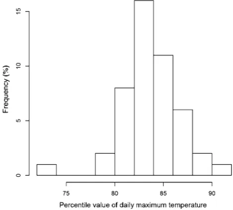
We obtained OT estimates for 47 prefectures in Japan using a smoothing spline with six degrees of freedom. As shown in Fig. 3, data points in the very hot range, espe-cially beyond 35°C, are sparse. Figure 4 shows the dis-tribution of percentile values that correspond to the OT. In most cases, the value was around the 84th percentile. The mean of all the 47 prefectures was the 83.6th percentile, and we used this value to estimate the OT.
Table2 presents the OT and 84th percentile value of daily maximum temperature in the cities of the other countries examined in this study. The OTs and 84th per-centile values were close to each other in a majority of the cities. There were 3 US cities (Dallas/Fort Worth, Houston, and San Diego) that did not show a V-shaped relation. These 3 cities are located in the south, and it is possible to speculate that air-conditioned houses are very popular in these hot cities such that residents of these cities have adapted to heat exposure. However, other southern cities showed a V-shaped relation, even when the OT was higher than 40°C. Also, in many mid- to southern Japanese pre-fectures, more than 90 % of households are equipped with air-conditioners (based on the 2009 National Survey of Family Income and Expenditure, for example), but these prefectures still showed V-shaped temperature–mortality relations. Hence, these 3 US cities may be exceptions due to statistical variation. From this multicountry examination, we concluded that OT can be estimated by the 83.6th percentile value of daily maximum temperature.
Precision improvement
To improve precision, use of long-term data and combining area-specific data are effective, provided that the Table 1 Description of mortality data by country
Country/ region
Observation period
Age category
Note
Japan 1972–2008 65? 47 prefectures, 1973–2008 for Okinawa
Korea 1992–2010 65? 6 cities
Taiwan 1994–2007 65? 3 cities
USA 1987–2000 65? 20 cities
Spain 1992–2000 All ages Barcelona
France 1991–1998 All ages Paris
chronological trend is well controlled and the heterogeneity among areas is reasonably small.
To control for chronological trend and population size, we introduced relative risk. The reference mortality for each year is the average number of deaths during the days with daily maximum temperature from the 75th to 85th percentile for each year. We chose this reference because this reference temperature range usually covers the OT, and because this reference is less affected by influenza epi-demic than the annual average daily number of deaths or adding time trend in regression models as a nonparametric term.
Lag effect inclusion
As explained earlier, lag effect should be controlled for to obtain the overall heat-related effect. For this purpose, we used a distributed lag nonlinear model [8]. In the actual calculation, we used the dlnm package developed by Gas-parrini [12] in R 2.15.1 [13]. In their paper, they describe dlnm as ‘‘a modelling framework that can simultaneously represent non-linear exposure–response dependencies and delayed effects. This methodology is based on the definition Fig. 3 Relation between daily maximum temperature and relative
risk (RR) in Tokyo, 1972–2008
Fig. 4 Distribution of optimum temperature (expressed as percentile value of daily maximum temperature) in Japan
Table 2 OT, 84th percentile ofTmax, and ratio of RMOTover RMav
Country City OT 84th percentile ofTmax
Ratio
Taiwan Taipei 33.4 33.9 0.95
Taichung 33.0 33.0 0.94
Kaohsiung 31.2 32.5 0.96
Korea Seoul 27.8 28.1 0.93
Busan 28.7 26.6 0.93
Daegu 29.9 29.5 0.93
Incheon 27.5 26.9 0.94
Gwangju 29.1 28.8 0.92
Daejeon 29.6 28.4 0.91
USA Los Angeles 30.0 28.3 0.95
New York 26.7 28.3 0.92
Chicago 26.1 27.8 0.94
Dallas/Fort Worthb 37.2 34.4 0.93
Houstonb 41.7 33.9 0.93
Phoenix 41.7 40.0 0.89
Santa Ana/Anaheim 33.3 31.1 0.94
San Diegob 41.7 24.4 0.95
Miami 31.7 32.2 0.96
Detroit 25.0 27.2 0.93
Seattle 22.2 23.3 0.93
San Bernardino 39.4 38.9 0.91
San Jose 30.6 31.7 0.91
Minneapolis/St. Paul 26.7 26.7 0.92
Riverside 44.4 42.8 0.91
Philadelphia 27.8 29.4 0.92
Atlanta 31.7 31.1 0.93
Oakland 32.8 33.9 0.90
Denver 33.3 32.2 0.92
Cleveland 26.1 26.7 0.94
Spain Barcelona 27.9 29.4 0.88a
France Paris 22.8 23.6 0.92a
Italy Rome 25.0 26.8 0.89a
a Target population is all ages combined
of a ‘cross-basis’, a bi-dimensional space of functions that describes simultaneously the shape of the relationship along both the space of the predictor and the lag dimension of its occurrence.’’ In our model, we used OT-offset daily maxi-mum temperature (expressed as ‘‘Tmax-OT’’) as the tem-perature index. Another choice would be the percentile value of daily maximum temperature, because most prefectures have OT close to the 84th percentile value. However, the range of daily maximum temperature is very wide in north-ern prefectures, whereas that in southnorth-ern prefectures is nar-row, so a one-unit increase of the percentile corresponds to a different increase in temperature.
The parameter setting of the dlnm model is as follows: For both OT-offset daily maximum temperature and its lag (from 0 to 15 days), we used natural cubic splines with degree of freedom 6. OT-offset daily maximum tempera-ture=0, i.e., the mortality level at OT, was used as a reference. Since we used relative mortality, quasi-Poisson distribution was assumed. Figure5shows the dlnm result.
This curve shows the result of adding up the lag effect. Figure6 shows the lag pattern for the situation when the daily maximum temperature is 5°C higher than OT. Lag 0 days had the highest risk, followed by lag 1 day. These risks, including slightly negative risk up to lag 15 days, were added up to construct Fig.5. As observed, heat-related mortality increases monotonically above OT. On the other hand, below OT there is a complex relationship between mortality and temperature.
From relative risk to excess number of deaths
The above risk function curve used the relative risk, and we need to estimate the excess number of deaths using this relative risk. Because the reference of the relative risk is the risk at OT, we can convert the relative risks if we can calculate the number of deaths when the temperature is the OT (NDOT). For this purpose, considering that the available information is the annual number of deaths (NAN), we need the following formula:
NDOT¼ðNAN=365:25Þ RMOT=RMav;
where RMOT is the relative risk at OT and RMav is the average daily relative risk. (NAN/365.25) yields the daily average number of deaths. We obtained both RMOT and RMav using the Japanese dataset. Based on the Japanese dataset, the average and standard deviation of RMOT/RMav were 0.88 and 0.014, respectively.
To examine the robustness of the above index, we used selected data from cities in Korea, Taiwan, the USA, and Europe. Table2 presents the values of this ratio in these countries selected for this manuscript. Although cities in Korea, Taiwan, and the USA showed a higher ratio than Japanese prefectures, two European countries showed a lower ratio. Considering that the European data are for all ages combined, the ratios for the 65?-year-old age group is expected to be even lower, because \65-year-old age groups are usually more resistant to heat; heat-related rel-ative risk is lower for younger age groups. Based on this observation, we decided to use the Japanese ratio, 0.88, for global projection.
Projection of future impact of climate change on heat-related mortality
We need the daily maximum temperature distribution for risk estimation. So, we chose NCC (= NCEP Corrected by CRU, where NCEP stands for National Centers for Envi-ronmental Prediction, USA, and CRU stands for Climate Research Unit, University of East Anglia) daily data [14] as the baseline climate data. For the future climates, we used one of the general circulation models provided by the WHO Global Burden of Diseases project, i.e., BCM2. Fig. 5 Risk function of excess mortality due to heat (for 47
prefectures in Japan, 1972–2008). Note: Lag effects up to 15 days were added to construct this curve
Here, we added the monthly average difference between the current climate and the future climate from models to each of the baseline daily maximum temperatures within the same month. The grid resolution is 1°. As the socio-economic scenario, we used SRES A1B.
Adaptation is another concern. When the OT is esti-mated as the 83.6th percentile value of daily maximum temperature as of the current climate, we assume no adaptation (0 % adaptation). If the future climate is used for OT estimation, we assume 100 % adaptation. The midpoint of the 0 and 100 % adaptation OTs is assumed to be the OT for 50 % adaptation. V-shape flattening is another possible type of adaptation, but our preliminary analyses showed no evidence of flattening (this will be published in another paper), and we did not include this type of adaptation in this manuscript.
Because there are excess deaths due to heat even at present, the excess number of deaths attributable to climate change is calculated using the ‘‘counterfactual method.’’ The idea is that, with identical annual mortality rate, what is the difference between the number of excess deaths in the baseline case and that in the altered climate case? The actual procedure for 2030 is as follows: The calculation was done for each 1°91° grid of the globe. We used the annual number of deaths (provided by the WHO) in 2030 for both the baseline and altered climate case. Then, for the baseline case, we applied the temperature distribution of the current climate (1961–1990) to the risk functions (based on 47 pre-fectures of Japan) for 0, 50, and 100 % adaptation; for the altered climate case, we applied the temperature distribution of the projected 2030 climate obtained using BCM2 instead of the current climate. The difference in the number of excess deaths between these two cases is considered to be the cli-mate-attributable excess number of deaths. These grid-spe-cific numbers of deaths were summed up for each WHO region (Table3). Likewise, the 2050 climate-attributable excess number of deaths was calculated.
Results
Table4 presents the projected excess heat-related deaths by WHO region. Asian regions are vulnerable to climate change impact.
In some regions, the heat-related excess deaths consti-tute up to 0.6 % of deaths, and some high-income regions also suffer a 0.1–0.4 % excess.
Discussion
Because this manuscript aims at developing a better pro-jection model for heat-related excess deaths, the problems
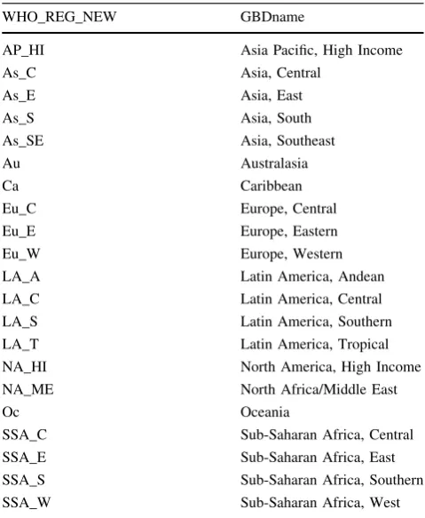
and their solutions were already addressed in ‘‘Materials and methods’’ section. Here, we evaluate how our goal was achieved, i.e., how much the fit, precision, and robustness of the proposed model have been improved from the pre-vious projection [7]. As shown in Figs. 2 and 5, it is obvious that the fit is much better for the present model. To show the improvement of precision, we used the present model and applied it to the observation period of the pre-vious model, i.e., 1972–1995. As an example, when the temperature was 10°C higher than OT, the risk estimate (95 % confidence interval) of this calculation was 1.241 (1.218–1.265), whereas the present calculation gave 1.173 (1.156–1.189); the range of the confidence interval was 30 % smaller. As for the robustness, Table2clearly shows the similarity of the OT and the ratio of RMOTover RMav across a wide range of areas, including Asia, the USA, and Europe. Hence, our model that sets OT to be around the 84th percentile value of daily maximum temperature can be generalizable to all over the world. One additional concern may be the applicability of our OT estimation to tropical areas, where the annual temperature difference is very small. Our analyses covered very cold areas to subtropical areas, but did not cover tropical areas or countries in the Southern Hemisphere. In this regard, McMichael and coworkers’ report [15] is worth mentioning, because they observed the heat-related effect for 12 cities including cities in tropical countries and those in the Southern Table 3 WHO regions
WHO_REG_NEW GBDname
AP_HI Asia Pacific, High Income
As_C Asia, Central
As_E Asia, East
As_S Asia, South
As_SE Asia, Southeast
Au Australasia
Ca Caribbean
Eu_C Europe, Central
Eu_E Europe, Eastern
Eu_W Europe, Western
LA_A Latin America, Andean
LA_C Latin America, Central
LA_S Latin America, Southern
LA_T Latin America, Tropical
NA_HI North America, High Income
NA_ME North Africa/Middle East
Oc Oceania
SSA_C Sub-Saharan Africa, Central
SSA_E Sub-Saharan Africa, East
SSA_S Sub-Saharan Africa, Southern
Hemisphere. Their model used a different method from ours; For example, they used daily mean temperature instead of daily maximum temperature, and they averaged out lag effect for lag 0–1 day and for lag 0–13 days. Still, the relation of the 0–1 averaged lag model was V-shaped for the majority of the cities. Considering that the 84th percentile value is roughly equal to the summer mean temperature, we tried to identify summer average temper-ature and optimum tempertemper-ature from the graphs they pro-vided. Among the cities with a V-shaped relation, most of the cities, including a tropical city (Bangkok, Thailand), had optimum temperature similar to their respective sum-mer average temperature. Although this procedure is not accurate, at least use of the 84th percentile value in pre-dicting OT cannot be falsified even by observations of cities in tropical zones or in the Southern Hemisphere. Another supporting report is the 4th Assessment Report of the Intergovernmental Panel on Climate Change [16]; temperature rise in tropical areas is expected to be less prominent compared with temperate areas and high-lati-tude areas. Hence, our projection would not be wide of the mark.
Compared with our previous projection, this new pro-jection has advantages in terms of fit, precision, and
robustness. Also, we included lag effect, which addresses mortality displacement. This implies that, although there may be some mortality displacement effect, the overall risk exists and climate change would increase the burden due to heat-related mortality.
Because the purpose of this paper is to show how we have improved the model for the global projection, we showed the projection results using only one global cir-culation model. However, the model described in this paper was adopted in the new WHO Global Burden of Diseases attributable to climate change, which will appear some-where soon, and several models will be used and compared.
Compared with the total number of deaths, the propor-tion of deaths due to heat-related mortality attributable to climate change appears small. However, considering that even huge cyclones do not kill many people nowadays in high-income countries, heat waves are a major environ-mental hazard. Of course, we need to compare the heat-related impact and cold-heat-related impact to obtain the net impact of global warming. However, new papers have warned that we should not naively apply the V-shaped temperature–mortality relation to projections for future cold-related excess deaths [17,18]. We will try to develop Table 4 Projection of heat-related excess deaths
Region 2030 2050
Populationa Baseline 0 %b 50 %b 100 %b Populationa Baseline 0 %b 50 %b 100 %b
AP_HI 177,053 2,427 4,802 3,635 2,598 162,307 2,528 6,866 4,395 2,588
As_C 9,529 611 1,458 975 598 103,588 947 3,797 2,024 854
As_E 1,428,481 5,343 18,423 11,053 5,837 1,332,115 7,050 36,739 18,612 7,184
As_S 2,033,885 10,692 26,666 18,022 11,296 2,284,943 17,429 65,562 37,524 18,489
As_SE 723,970 1,449 5,718 3,078 1,594 777,181 2,487 19,662 8,371 2,549
Au 32,982 119 370 230 125 37,063 156 837 424 174
Ca 48,633 2 195 75 2 49,792 3 553 261 3
Eu_C 115,732 988 3,123 1,955 1,090 107,099 1,058 5,396 2,998 1,417
Eu_E 195,411 1,708 6,350 3,647 1,860 178,872 1,732 10,471 4,845 1,721
Eu_W 441,260 3,570 6,214 4,722 3,485 446,713 4,425 13,367 8,334 4,677
LA_A 66,776 41 372 160 40 75,150 71 1,760 548 78
LA_C 287,206 700 2,181 1,239 711 318,626 1,226 7,364 3,363 1,249
LA_S 69,901 234 924 537 263 74,285 301 2,069 925 289
LA_T 229,162 364 2,050 1,066 432 233,166 563 6,546 2,545 694
NA_HI 401,536 2,408 7,394 4,704 2,702 446,749 2,953 15,441 7,877 3,235
NA_ME 584,318 1,596 4,780 2,977 1,683 681,137 3,209 15,331 7,940 3,302
Oc 14,113 4 47 14 3 18,172 8 195 68 7
SSA_C 152,539 201 918 482 221 212,327 438 4,007 1,645 485
SSA_E 574,918 858 3,686 1,923 857 848,878 1,679 14,734 6,060 1,776
SSA_S 81,752 156 539 319 165 87,940 246 1,737 798 300
SSA_W 543,556 775 2,491 1,486 785 809,872 1,578 9,468 4,465 1,679
a In thousands. Based on United Nations 2010 revision, medium estimates
our model for cold-related excess mortality after taking into account the points these papers raised in the near future.
Acknowledgments This study was supported by the Environment Research and Technology Development Fund (S-8 & S10) of the Ministry of the Environment, Japan, and the Global Research Labo-ratory (grant K21004000001-10A0500-00710) through the National Research Foundation of Korea (NRF), funded by the Ministry of Education, Science, and Technology, Korea.
Conflict of interest All authors have no conflicts of interest.
References
1. WHO. The World Health Report 2002-reducing risks, promoting healthy life. Geneva: WHO; 2002.
2. Kunst AE, Looman CW, Mackenbach JP. Outdoor air tempera-ture and mortality in the Netherlands: a time-series analysis. Am J Epidemiol. 1993;137:331–41.
3. El-Zein A, Tewtel-Salem M, Nehme G. A time-series analysis of mortality and air temperature in Greater Beirut. Sci Total Envi-ron. 2004;330:71–80.
4. Honda Y, Ono M, Sasaki A, Uchiyama I. Shift of the short-term temperature mortality relationship by a climate factor—some evidence necessary to take account of in estimating the health effect of global warming. J Risk Res. 1998;1:209–20.
5. Curriero FC, Heiner KS, Samet JM, Zeger SL, Strug L, Patz J a. Temperature and mortality in 11 cities of the eastern United States. Am J Epidemiol. 2002;155:80–7.
6. Honda Y, Kabuto M, Ono M, Uchiyama I. Determination of optimum daily maximum temperature using climate data. Envi-ron Health Prev Med. 2007;12:209–16.
7. Takahashi K, Honda Y, Emori S. Assessing mortality risk from heat stress due to global warming. J Risk Res. 2007;10:339–54. 8. Armstrong B. Models for the relationship between ambient
temperature and daily mortality. Epidemiology. 2006;17:624–31. 9. Fouillet A, Rey G, Laurent F, Pavillon G, Bellec S, Guihenneuc-Jouyaux C, et al. Excess mortality related to the August 2003 heat wave in France. Int Arch Occup Environ Health. 2006;80:16–24. 10. Bell ML, Dominici F, Samet JM. A meta-analysis of time-series studies of ozone and mortality with comparison to the national morbidity, mortality, and air pollution study. Epidemiology. 2005;16:436–45.
11. Mathers CD, Loncar D. Projections of global mortality and bur-den of disease from 2002 to 2030. PLoS Med. 2006;3:e442. 12. Gasparrini A, Armstrong B, Kenward MG. Distributed lag
non-linear models. Stat Med. 2010;29:2224–34.
13. Ihaka R, Gentleman RR. A language for data analysis and graphics. J Comput Graph Stat. 1996;5:299–314.
14. Ngo-Duc T. A 53-year forcing data set for land surface models. J Geophys Res. 2005;110:D06116.
15. McMichael AJ, Wilkinson P, Kovats RS, Pattenden S, Hajat S, Armstrong B, et al. International study of temperature, heat and urban mortality: the ‘‘ISOTHURM’’ project. Int J Epidemiol. 2008;37:1121–31.
16. Solomon S, Qin D, Manning M, Chen Z, Marquis M, Ave KB. IPCC. Summary for Policymakers. In: Climate Change 2007. The physical science basis contribution of working group I to the fourth assessment report of the intergovernmental panel on cli-mate change. Cambridge, UK and New York, USA: Cambridge University Press; 2007. p 18.
17. Kinney PL, Pascal M, Vautard R, Laaidi K. Winter mortality in a changing climate: will it go down? Bull Epide´miol Hebd. 2012;12–13:148–51.