186
Chapter
A
n automobile’s gas mileage is a function of
many variables, including road surface, tire
type, velocity, fuel octane rating, road angle,
and the speed and direction of the wind. If we look
only at velocity’s effect on gas mileage, the mileage
of a certain car can be approximated by:
m(v)
0.00015v
30.032v
21.8v
1.7
(where v
is velocity)
At what speed should you drive this car to
ob-tain the best gas mileage? The ideas in Section 4.1
will help you find the answer.
Applications of
Derivatives
Section 4.1 Extreme Values of Functions 187
Chapter 4 Overview
In the past, when virtually all graphing was done by hand—often laboriously—derivatives
were the key tool used to sketch the graph of a function. Now we can graph a function
quickly, and usually correctly, using a grapher. However, confirmation of much of what we
see and conclude true from a grapher view must still come from calculus.
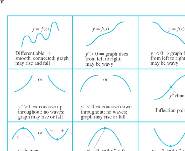
This chapter shows how to draw conclusions from derivatives about the extreme
val-ues of a function and about the general shape of a function’s graph. We will also see
how a tangent line captures the shape of a curve near the point of tangency, how to
de-duce rates of change we cannot measure from rates of change we already know, and
how to find a function when we know only its first derivative and its value at a single
point. The key to recovering functions from derivatives is the Mean Value Theorem, a
theorem whose corollaries provide the gateway to
integral calculus,
which we begin in
Chapter 5.
Extreme Values of Functions
Absolute (Global) Extreme Values
One of the most useful things we can learn from a function’s derivative is whether the
function assumes any maximum or minimum values on a given interval and where
these values are located if it does. Once we know how to find a function’s extreme
val-ues, we will be able to answer such questions as “What is the most effective size for a
dose of medicine?” and “What is the least expensive way to pipe oil from an offshore
well to a refinery down the coast?” We will see how to answer questions like these in
Section 4.4.
4.1
What you’ll learn about
• Absolute (Global) Extreme Values
• Local (Relative) Extreme Values
• Finding Extreme Values
. . . and why
Finding maximum and minimum
values of functions, called
opti-mization, is an important issue in
real-world problems.
DEFINITION
Absolute Extreme Values
Let
f
be a function with domain
D.
Then
f
c
is the
(a) absolute maximum value
on
D
if and only if
f
x
f
c
for all
x
in
D.
(b) absolute minimum value
on
D
if and only if
f
x
f
c
for all
x
in
D.
Absolute (or
global
) maximum and minimum values are also called
absolute extrema
(plural of the Latin
extremum
). We often omit the term “absolute” or “global” and just say
maximum and minimum.
Example 1 shows that extreme values can occur at interior points or endpoints of
intervals.
EXAMPLE 1
Exploring Extreme Values
On
p
2,
p
2
,
f
x
cos
x
takes on a maximum value of 1 (once) and a minimum
value of 0 (twice). The function
g
x
sin
x
takes on a maximum value of 1 and a
minimum value of
1 ( Figure 4.1).
Now try Exercise 1.Functions with the same defining rule can have different extrema, depending on the
domain.
Figure 4.1 (Example 1)
x y
0 1
–1
y sin x
–– 2 –
y cos x
EXAMPLE 2
Exploring Absolute Extrema
The absolute extrema of the following functions on their domains can be seen in Figure 4.2.
Function Rule Domain D Absolute Extrema on D
(a) yx2 , No absolute maximum.
Absolute minimum of 0 at x0.
(b) yx2 0, 2 Absolute maximum of 4 at x2.
Absolute minimum of 0 at x0.
(c) yx2 0, 2 Absolute maximum of 4 at x2.
No absolute minimum.
(d) yx2 0, 2 No absolute extrema.
Now try Exercise 3.
Example 2 shows that a function may fail to have a maximum or minimum value. This
cannot happen with a continuous function on a finite closed interval.
THEOREM 1
The Extreme Value Theorem
If
f
is continuous on a closed interval
a
,
b
, then
f
has both a maximum value and a
minimum value on the interval. ( Figure 4.3)
Figure 4.2 (Example 2)
x y
2
(a) abs min only
yx2 D (–, )
x y
2
(b) abs max and min
yx2
D [0, 2]
x y
2
(c) abs max only
yx2 D (0, 2]
x y
2
(d) no abs max or min
yx2 D (0, 2)
Figure 4.3 Some possibilities for a continuous function’s maximum (M) and minimum (m) on a closed interval [a,b].
x a
yf(x) (x2, M)
Maximum and minimum at interior points
x2 b
M
x1
(x1, m)
m
x
a b
yf(x)
M
m
Maximum and minimum at endpoints
x a
yf(x)
Maximum at interior point, minimum at endpoint
x2 M
b m
x a
yf(x)
Minimum at interior point, maximum at endpoint
x1
M
Section 4.1 Extreme Values of Functions 189
Local (Relative) Extreme Values
Figure 4.4 shows a graph with five points where a function has extreme values on its domain
a
,
b
. The function’s absolute minimum occurs at
a
even though at
e
the function’s value is
smaller than at any other point
nearby.
The curve rises to the left and falls to the right around
c
, making
f
c
a maximum locally. The function attains its absolute maximum at
d.
THEOREM 2
Local Extreme Values
If a function
f
has a local maximum value or a local minimum value at an interior
point
c
of its domain, and if
f
exists at
c
, then
f
c
0.
Local extrema are also called
relative extrema.
An
absolute extremum
is also a local extremum, because being an extreme value
overall makes it an extreme value in its immediate neighborhood. Hence,
a list of local
ex-trema will automatically include absolute exex-trema if there are any.
Finding Extreme Values
The interior domain points where the function in Figure 4.4 has local extreme values are
points where either
f
is zero or
f
does not exist. This is generally the case, as we see from
the following theorem.
Figure 4.4 Classifying extreme values.
x b
a
yf(x)
c e d
Local maximum. No greater value of
f nearby.
Absolute maximum. No greater value of f anywhere. Also a local maximum.
Local minimum. No smaller value of
f nearby.
Local minimum. No smaller value of f nearby.
Absolute minimum. No smaller value of f anywhere. Also a local minimum.
DEFINITION
Local Extreme Values
Let
c
be an interior point of the domain of the function
f.
Then
f
c
is a
(a) local maximum value
at
c
if and only if
f
x
f
c
for all
x
in some open
interval containing
c.
(b) local minimum value
at
c
if and only if
f
x
f
c
for all
x
in some open
interval containing
c.
EXAMPLE 3
Finding Absolute Extrema
Find the absolute maximum and minimum values of
f
x
x
23on the interval
2, 3
.
SOLUTION
Solve Graphically
Figure 4.5 suggests that
f
has an absolute maximum value of
about 2 at
x
3 and an absolute minimum value of 0 at
x
0.
Confirm Analytically
We evaluate the function at the critical points and endpoints
and take the largest and smallest of the resulting values.
The first derivative
f
x
2
3
x
13
3
2
3
x
has no zeros but is undefined at
x
0. The values of
f
at this one critical point and at
the endpoints are
Critical point value:
f
0
0;
Endpoint values:
f
2
2
233
4
;
f
3
3
233
9
.
We can see from this list that the function’s absolute maximum value is
39
2.08,
and occurs at the right endpoint
x
3. The absolute minimum value is 0, and occurs
at the interior point
x
0.
Now try Exercise 11.In Example 4, we investigate the reciprocal of the function whose graph was drawn in
Example 3 of Section 1.2 to illustrate “grapher failure.”
EXAMPLE 4
Finding Extreme Values
Find the extreme values of
f
x
4
1
x
2.
SOLUTIONSolve Graphically
Figure 4.6 suggests that
f
has an absolute minimum of about 0.5 at
x
0. There also appear to be local maxima at
x
2 and
x
2. However,
f
is not
de-fined at these points and there do not appear to be maxima anywhere else.
continued
Figure 4.5 (Example 3)
[–2, 3] by [–1, 2.5]
yx2/3
Figure 4.6 The graph of
fx 4
1
x2.
(Example 4)
[–4, 4] by [–2, 4]
Because of Theorem 2, we usually need to look at only a few points to find a function’s
extrema. These consist of the interior domain points where
f
0 or
f
does not exist (the
domain points covered by the theorem) and the domain endpoints (the domain points not
covered by the theorem). At all other domain points,
f
0 or
f
0.
The following definition helps us summarize these findings.
Thus, in summary, extreme values occur only at critical points and endpoints.
DEFINITION
Critical Point
Section 4.1 Extreme Values of Functions 191
Confirm Analytically
The function
f
is defined only for 4
x20, so its domain
is the open interval
2, 2
. The domain has no endpoints, so all the extreme values
must occur at critical points. We rewrite the formula for
f
to find
f
:
f
x
4
1
x
24
x
2
12
.
Thus,
f
x
1
2
4
x
2
3/2
2
x
4
x
x
232
.
The only critical point in the domain
2, 2
is
x
0. The value
f
0
4
1
0
21
2
is therefore the sole candidate for an extreme value.
To determine whether 1
2 is an extreme value of
f
, we examine the formula
f
x
4
1
x
2.
As
x
moves away from 0 on either side, the denominator gets smaller, the values of
f
increase, and the graph rises. We have a minimum value at
x
0, and the minimum is
absolute.
The function has no maxima, either local or absolute. This does not violate Theorem 1
( The Extreme Value Theorem) because here
f
is defined on an
open
interval. To invoke
Theorem 1’s guarantee of extreme points, the interval must be closed.
Now try Exercise 25.
While a function’s extrema can occur only at critical points and endpoints, not every
critical point or endpoint signals the presence of an extreme value. Figure 4.7 illustrates
this for interior points. Exercise 55 describes a function that fails to assume an extreme
value at an endpoint of its domain.
Figure 4.7 Critical points without extreme values. (a) y 3x2is 0 at
x
0, butyx3has no extremum there. (b) y 1
3x23is undefined at x0, but yx13has no extremum there.
–1
x y
1 –1
1
yx3
0
(a)
–1
x y
1 –1
1
yx1/3
(b)
EXAMPLE 5
Finding Extreme Values
Find the extreme values of
5
2
x
2,
x
1
f
x
{
x
2,
x
1.
SOLUTION
Solve Graphically
The graph in Figure 4.8 suggests that
f
0
0 and that
f
1
does not exist. There appears to be a local maximum value of 5 at
x
0 and a local
minimum value of 3 at
x
1.
Confirm Analytically
For
x
1, the derivative is
f
x
{
d
d
x
5
2
x
24
x
,
x
1
d
d
x
x
2
1,
x
1.
The only point where
f
0 is
x
0. What happens at
x
1?
At
x
1, the right- and left-hand derivatives are respectively
lim
h→0
f
1
h
h
f
1
lim
h→0
1
h
h
2
3
lim
h→0h
h
1,
lim
h→0
f
1
h
h
f
1
lim
h→0
5
2
1
h
h
23
lim
h→0
2
h
h
2
h
4.
Since these one-sided derivatives differ,
f
has no derivative at
x
1, and 1 is a second
critical point of
f.
The domain
,
has no endpoints, so the only values of
f
that might be local
ex-trema are those at the critical points:
f
0
5
and
f
1
3.
From the formula for
f
, we see that the values of
f
immediately to either side of
x
0
are less than 5, so 5 is a local maximum. Similarly, the values of
f
immediately to either
side of
x
1 are greater than 3, so 3 is a local minimum.
Now try Exercise 41.Most graphing calculators have built-in methods to find the coordinates of points where
extreme values occur. We must, of course, be sure that we use correct graphs to find these
values. The calculus that you learn in this chapter should make you feel more confident
about working with graphs.
EXAMPLE 6
Using Graphical Methods
Find the extreme values of
f
x
ln
1
x
x
2.
SOLUTIONSolve Graphically
The domain of
f
is the set of all nonzero real numbers. Figure 4.9
suggests that
f
is an even function with a maximum value at two points. The coordinates
found in this window suggest an extreme value of about
0.69 at approximately
x
1. Because
f
is even, there is another extreme of the same value at approximately
x
1. The figure also suggests a minimum value at
x
0, but
f
is not defined
there.
Confirm Analytically
The derivative
f
x
x
1
1
x
x
2
2
is defined at every point of the function’s domain. The critical points where
f
x
0 are
x
1 and
x
1. The corresponding values of
f
are both ln
1
2
ln 2
0.69.
Now try Exercise 37.
Figure 4.8 The function in Example 5.
[–5, 5] by [–5, 10]
Figure 4.9 The function in Example 6.
[–4.5, 4.5] by [–4, 2]
Maximum
Section 4.1 Extreme Values of Functions 193
Section 4.1 Exercises
Finding Extreme Values
Let
f
x
x
2x
1
,
2
x
2.
1.
Determine graphically the extreme values of
f
and where they occur. Find
f
at
these values of
x.
2.
Graph
f
and
f
or NDER
f
x
,
x, x
in the same viewing window. Comment
on the relationship between the graphs.
3.
Find a formula for
f
x
.
EXPLORATION 1
In Exercises 1–4, find the first derivative of the function.
1. fx4x 2. fx
9 2
x2 (9 2 x x
2)3/2
3. gxcos ln x sin ( x
lnx)
4. hxe2x 2e2x
In Exercises 5–8, match the table with a graph of f(x).
5. 6.
7. 8.
In Exercises 9 and 10, find the limit for
fx 9
2
x2.
9. lim
x→3fx 10.x→lim3fx
In Exercises 11 and 12, let
x32x, x2
fx
{
x2, x2.
11. Find (a)f 1, 1 (b)f 3, 1 (c)f 2. Undefined
12. (a)Find the domain off . x2
(b)Write a formula forf x. f (x)
3x22,x2 1,x2a b c
(d)
a b c
(c)
a b c
(b)
a b c
(a)
x fx
a does not exist
b does not exist
c 1.7
x f x
a does not exist
b 0
c 2
x fx
a 0
b 0
c 5
x f x
a 0
b 0
c 5
Quick Review 4.1
(For help, go to Sections 1.2, 2.1, 3.5, and 3.6.)
In Exercises 1–4, find the extreme values and where they occur.
1. 2.
x y
1 –1
1
–1
x y
2 2
–2 0
3. 4.
2 (1, 2)
–1
–3 2 x
y
x y
0 2
5
1
24x
(c) (b)
(d) (a)
1.Minima at (2, 0) and (2, 0), maximum at (0, 2)
2.Local minimum at (1, 0), local maximum at (1, 0)
3.Maximum at (0, 5)
In Exercises 5–10, identify each x-value at which any absolute ex-treme value occurs. Explain how your answer is consistent with the Extreme Value Theorem. See page 195.
5. 6.
7. 8.
9. 10.
In Exercises 11–18, use analytic methods to find the extreme values of the function on the interval and where they occur. See page 195.
11. fx 1
x ln x, 0.5x4 12. gxex, 1x1
13. hxln x1, 0x3
14. kxex2
, x
15. fxsin
(
x p4
)
, 0x 74
p
16. gxsec x, p 2 x
3 2
p
17. fxx25, 3x1
18. fxx35, 2x3
In Exercises 19–30, find the extreme values of the function and where they occur.
19. y2x28x9 20. yx32x4
21. yx3x28x5 22. yx33x23x2
23. yx21 24. y
x2 1 1 25. y 1 1
x2 26. y 3
1
1
x2
27. y32xx2
28. y 3
2x
44x39x210
29. y x2 x 1 30. y x2 x 2x 1 2 x y
0 a c b
yg(x)
x y
0 a c b
yg(x)
x y
0 a b
yh(x)
c x
y
0 a b
yf(x)
c
x y
0 a c b
yf(x)
x y
0 a c1 b
yh(x)
c2
Group Activity In Exercises 31–34, find the extreme values of the function on the interval and where they occur.
31. fx x2 x3, 5x5
32. gx x1 x5, 2x7
33. hx x2 x3, x 34. kx x1 x3, x
In Exercises 35–42, identify the critical point and determine the local extreme values.
35. yx23x2 36.yx23x24
37. yx4x2 38.yx23x
39. y
{
42x, x1 x1, x140. y
{
3x, x032xx2, x0
41. x
22x4, x1
y
{
x26x4, x1
1 4x 2 1 2x 1 4 5
, x1
42. y
{
x36x28x, x1
43. Writing to Learn The function
Vxx102x162x, 0x5, models the volume of a box.
(a)Find the extreme values of V.
(b)Interpret any values found in (a) in terms of volume of the box.
44. Writing to Learn The function
Px2x 20 x
0
, 0x ,
models the perimeter of a rectangle of dimensions xby 100
x. (a)Find any extreme values of P.(b)Give an interpretation in terms of perimeter of the rectangle for any values found in (a).
Standardized Test Questions
You should solve the following problems without using a graphing calculator.
45. True or False If f(c) is a local maximum of a continuous function fon an open interval (a,b), then f (c)0. Justify your answer.
46. True or False If mis a local minimum and Mis a local maxi-mum of a continuous function fon (a,b), then mM. Justify your answer.
47. Multiple Choice Which of the following values is the ab-solute maximum of the function f(x)4xx26 on the interval
[0, 4]? E
(A)0 (B)2 (C)4 (D)6 (E)10
45.False. For example, the maximum could occur at a corner, where f (c) would not exist.
Min value 1 at x2
Min value 1 at x0
Max value 2 at x1; min value 0 at x 1, 3 Min value 0
at x 1, 1
None
Local max at (0,1)
Local min at (0, 1)
21.Local max at (2, 17); local min at
4 3,4 2 1 7
Max value is 144 at x2.
Min value is 40 at x10. The largest volume of the box is 144 cubic units and it occurs when x 2.
Section 4.1 Extreme Values of Functions 195
48. Multiple Choice If fis a continuous, decreasing function on [0, 10] with a critical point at (4, 2), which of the following state-ments must be false? E
(A)f(10) is an absolute minimum of fon [0, 10].
(B)f(4) is neither a relative maximum nor a relative minimum.
(C)f (4) does not exist.
(D) f (4)0
(E) f (4)0
49. Multiple Choice Which of the following functions has exactly two local extrema on its domain? B
(A)f(x)⏐x2⏐
(B)f(x)x36x5
(C)f(x) x3 6x 5
(D)f(x)tan x (E)f(x)xln x
50. Multiple Choice If an even function f with domain all real numbers has a local maximum at xa, then f(a) B
(A)is a local minimum.
(B)is a local maximum.
(C)is both a local minimum and a local maximum.
(D)could be either a local minimum or a local maximum.
(E)is neither a local minimum nor a local maximum.
Explorations
In Exercises 51 and 52, give reasons for your answers.
51. Writing to Learn Let fxx223.
(a)Does f 2exist? No
(b)Show that the only local extreme value offoccurs at x2.
(c)Does the result in (b) contradict the Extreme Value Theorem?
(d)Repeat parts (a) and (b) for fxxa23, replacing 2 by a.
52. Writing to Learn Let fx x39x.
(a) Does f 0 exist? No (b)Does f 3 exist? No
(c)Does f 3 exist? No (d)Determine all extrema off.
Extending the Ideas
53. Cubic Functions Consider the cubic function
fxax3bx2cxd.
(a)Show thatfcan have 0, 1, or 2 critical points. Give examples and graphs to support your argument.
(b)How many local extreme values canfhave? Two or none
54. Proving Theorem 2 Assume that the functionfhas a local maximum value at the interior point cof its domain and that f(c) exists.
(a)Show that there is an open interval containing csuch that
fxfc0 for all xin the open interval.
(b)Writing to Learn Now explain why we may say
lim
x→c fx
x
c fc
0.
(c)Writing to Learn Now explain why we may say
lim
x→c fx
x
c fc
0.
(d)Writing to Learn Explain how parts (b) and (c) allow us to conclude f c0.
(e)Writing to Learn Give a similar argument iffhas a local minimum value at an interior point.
55. Functions with No Extreme Values at Endpoints
(a)Graph the function sin1
x, x0 fx
{
0, x0.
Explain why f0
0 is not a local extreme value off.(b)Group Activity Construct a function of your own that fails to have an extreme value at a domain endpoint.
Answers:
5.Maximum at xb, minimum at xc2;
Extreme Value Theorem applies, so both the max and min exist.
6.Maximum at xc, minimum at xb; Extreme Value Theorem applies, so both the max and min exist.
7.Maximum at xc, no minimum;
Extreme Value Theorem doesn’t apply, since the function isn’t defined on a closed interval.
8.No maximum, no minimum;
Extreme Value Theorem doesn’t apply, since the function isn’t continuous or defined on a closed interval.
9.Maximum at xc, minimum at xa; Extreme Value Theorem doesn’t apply, since the function isn’t continuous.
10.Maximum at xa, minimum at xc; Extreme Value Theorem doesn’t apply, since the function isn’t continuous.
11.Maximum value is 1
4 ln 4 at x4; minimum value is 1 at x1; local maximum at
12, 2ln 2
12.Maximum value is eat x 1; minimum value is 1 eat x1.
13.Maximum value is ln 4 at x3; minimum value is 0 at x0.
14.Maximum value is 1 at x0
15.Maximum value is 1 at x
4; minimum value is 1 at x 5
4;
local minimum at
0, ; local maximum at 7 4, 016.Local minimum at (0, 1); local maximum at (,1)
17.Maximum value is 32/5at x 3; minimum value is 0 at x0
18.Maximum value is 33/5at x3
1
2
51. (b)The derivative is defined and nonzero for x2. Also,f(2)0, and f(x)0 for all x2.
(c)No, because (,) is not a closed interval.
(d)The answers are the same as (a) and (b) with 2 replaced by a. Minimum value is 0 at x 3,
Mean Value Theorem
Mean Value Theorem
The Mean Value Theorem connects the average rate of change of a function over an interval
with the instantaneous rate of change of the function at a point within the interval. Its
pow-erful corollaries lie at the heart of some of the most important applications of the calculus.
The theorem says that somewhere between points
A
and
B
on a differentiable curve,
there is at least one tangent line parallel to chord
AB
( Figure 4.10).
The hypotheses of Theorem 3 cannot be relaxed. If they fail at even one point, the
graph may fail to have a tangent parallel to the chord. For instance, the function
f
x
x
is continuous on
1, 1
and differentiable at every point of the interior
1, 1
except
x
0. The graph has no tangent parallel to chord
AB
( Figure 4.11a). The function
g
x
int
x
is differentiable at every point of
1, 2
and continuous at every point of
1, 2
except
x
2. Again, the graph has no tangent parallel to chord
AB
( Figure 4.11b).
The Mean Value Theorem is an
existence theorem.
It tells us the number
c
exists
without telling how to find it. We can sometimes satisfy our curiosity about the value of
c
but the real importance of the theorem lies in the surprising conclusions we can draw
from it.
4.2
What you’ll learn about
• Mean Value Theorem
• Physical Interpretation
• Increasing and Decreasing
Functions
• Other Consequences
. . . and why
The Mean Value Theorem is an
important theoretical tool to
connect the average and
in-stantaneous rates of change.
Figure 4.10 Figure for the Mean Value Theorem.
x y
0
Slope f '(c)
a
Tangent parallel to chord
c b
yf(x)
Slope————–f(b) f(a)
ba B
A
THEOREM 3
Mean Value Theorem for Derivatives
If
y
f
x
is continuous at every point of the closed interval
a
,
b
and
differen-tiable at every point of its interior
a
,
b
, then there is at least one point
c
in
a
,
b
at
which
f
c
f
b
b
f
a
a
.
Rolle’s Theorem
The first version of the Mean Value The-orem was proved by French mathemati-cian Michel Rolle (1652–1719). His ver-sion had fafb0 and was proved only for polynomials, using algebra and geometry.
Rolle distrusted calculus and spent most of his life denouncing it. It is ironic that he is known today only for an unintended contribution to a field he tried to suppress.
y
x
0
f ' (c) = 0
a
y = f (x)
c b
Figure 4.11 No tangent parallel to chord AB.
x y
B (1, 1)
b 1
a –1
(a)
A (–1, 1)
y |x|, –1 ≤ x ≤ 1
y
x y int x, 1≤x ≤ 2
A (1, 1)
B (2, 2)
b 2
a 1
(b) 2
1
0
EXAMPLE 1
Exploring the Mean Value Theorem
Show that the function
f
x
x
2satisfies the hypotheses of the Mean Value Theorem
on the interval
0, 2
. Then find a solution
c
to the equation
f
c
f
b
b
f
a
a
on this interval.
Section 4.2 Mean Value Theorem 197
SOLUTION
The function
f
x
x
2is continuous on
0, 2
and differentiable on
0, 2
. Since
f
0
0 and
f
2
4, the Mean Value Theorem guarantees a point
c
in the interval
0, 2
for which
f
c
f
b
b
f
a
a
2
c
f
2
2
0
f
0
2 f
x2xc
1.
Interpret
The tangent line to
f
x
x
2at
x
1 has slope 2 and is parallel to the
chord joining
A
0, 0
and
B
2, 4
( Figure 4.12).
Now try Exercise 1.
EXAMPLE 2
Exploring the Mean Value Theorem
Explain why each of the following functions fails to satisfy the conditions of the Mean
Value Theorem on the interval [–1, 1].
(a)
f
(
x
)
x
21
(b)SOLUTION
(a)
Note that
x
2
1
|
x
|
1, so this is just a vertical shift of the absolute value
function, which has a nondifferentiable “corner” at
x
0. (See Section 3.2.) The
function
f
is not differentiable on (–1, 1).
(b)
Since lim
x→1–f(x)lim
x→1–x3 3 4 andlim
x→1+f(x)lim
x→1+x2 1 2,the
function has a discontinuity at
x
1. The function
f
is not continuous on [–1, 1].
If the two functions given had satisfied the necessary conditions, the
conclusion
of the
Mean Value Theorem would have guaranteed the existence of a number
c
in (– 1, 1)
such that
f
(
c
)
f
(1
1
)
(
f
(
1)
1)
0. Such a number
c
does not exist for the function in
part (a), but one happens to exist for the function in part (b) (Figure 4.13).
Figure 4.12 ( Example 1)
y = x2
x y
1 (1, 1)
B(2, 4)
A(0, 0) 2
Figure 4.13 For both functions in Example 2,f(1 1
)
(
f
( 1) 1)
0 but neither function satisfies the conditions of the Mean Value Theorem on the interval [– 1, 1]. For the function in Example 2(a), there is no number csuch that
f(c) 0. It happens that f(0) 0 in Example 2(b).
y
x
1 2 3
1 2
–1
–2 0
(a)
y
(b)
x
– 4
4
0 4
x
33 for
x
1
f
x
{
x
21 for
x
1
EXAMPLE 3
Applying the Mean Value Theorem
Let
f
x
1
x
2,
A
1,
f
1
, and
B
1,
f
1
. Find a
tangent to
f
in the interval
1, 1
that is parallel to the secant
AB.
SOLUTION
The function
f
(Figure 4.14) is continuous on the interval [–1, 1] and
f
x
1
x
x
2is defined on the interval
1, 1
. The function is not differentiable at
x
1 and
x
1,
but it does not need to be for the theorem to apply. Since
f
1
f
1
0, the tangent
we are looking for is horizontal. We find that
f
0 at
x
0, where the graph has the
horizontal tangent
y
1.
Now try Exercise 9.Physical Interpretation
If we think of the difference quotient
f
b
f
a
b
a
as the average change in
f
over
a
,
b
and
f
c
as an instantaneous change, then the Mean Value Theorem says that
the instantaneous change at some interior point must equal the average change over the
en-tire interval.
EXAMPLE 4
Interpreting the Mean Value Theorem
If a car accelerating from zero takes 8 sec to go 352 ft, its average velocity for the 8-sec
interval is 352
8
44 ft
sec, or 30 mph. At some point during the acceleration, the
the-orem says, the speedometer must read exactly 30 mph ( Figure 4.15).
Now try Exercise 11.
Increasing and Decreasing Functions
Our first use of the Mean Value Theorem will be its application to increasing and
decreas-ing functions.
Figure 4.15 ( Example 4)
Figure 4.14 ( Example 3)
y
x y
0 1
–1
1 x2
√⎯⎯⎯⎯⎯⎯
1 , –1 ≤ x 1≤
t s
0
5 80
160 At this point, the car’s speed was 30 mph.
Time (sec) (8, 352)
240 320 400
Distance (ft)
sf(t)
Monotonic Functions
A function that is always increasing on an interval or always decreasing on an interval is said to be monotonicthere.
The Mean Value Theorem allows us to identify exactly where graphs rise and fall.
Functions with positive derivatives are increasing functions; functions with negative
deriv-atives are decreasing functions.
COROLLARY
1 Increasing and Decreasing Functions
Let
f
be continuous on
a
,
b
and differentiable on
a
,
b
.
1.
If
f
0 at each point of
a
,
b
, then
f
increases on
a
,
b
.
2.If
f
0 at each point of
a
,
b
, then
f
decreases on
a
,
b
.
DEFINITIONS
Increasing Function, Decreasing Function
Let
f
be a function defined on an interval
I
and let
x
1and
x
2be any two points in
I.
Section 4.2 Mean Value Theorem 199
Proof
Let
x
1and
x
2be any two points in
a
,
b
with
x
1x
2. The Mean Value Theorem
applied to
f
on
x
1,
x
2gives
f
x
2f
x
1f
c
x
2x
1for some
c
between
x
1and
x
2. The sign of the right-hand side of this equation is the same
as the sign of
f
c
because
x
2x
1is positive. Therefore,
(a)
f
x
1f
x
2if
f
0 on
a
,
b
(
f
is increasing), or
(b)
f
x
1f
x
2if
f
0 on
a
,
b
(
f
is decreasing).
■
EXAMPLE 5
Determining Where Graphs Rise or Fall
The function
y
x
2( Figure 4.16) is
(a)
decreasing on
, 0
because
y
2
x
0 on
, 0
.
(b)
increasing on
0,
because
y
2
x
0 on
0,
.
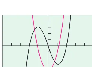
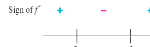
Now try Exercise 15.EXAMPLE 6
Determining Where Graphs Rise or Fall
Where is the function
f
x
x
34
x
increasing and where is it decreasing?
SOLUTIONSolve Graphically
The graph of
f
in Figure 4.17 suggests that
f
is increasing from
to the
x
-coordinate of the local maximum, decreasing between the two local
ex-trema, and increasing again from the
x
-coordinate of the local minimum to
. This
in-formation is supported by the superimposed graph of
f
x
3
x
24.
Confirm Analytically
The function is increasing where
f
x
0.
3
x
24
0
x
24
3
x
4
3
or
x
4
3
The function is decreasing where
f
x
0.
3
x
24
0
x
24
3
4
3
x
4
3
In interval notation,
f
is increasing on
,
4
3
], decreasing on
4
3
,
4
3
,
and increasing on
4
3
,
.
Now try Exercise 27.Other Consequences
[image:14.684.47.200.428.539.2]We know that constant functions have the zero function as their derivative. We can now
use the Mean Value Theorem to show conversely that the only functions with the zero
function as derivative are constant functions.
Figure 4.16 ( Example 5)
Figure 4.17 By comparing the graphs of
f
x
x34xandfx3x24wecan relate the increasing and decreasing behavior offto the sign off. ( Example 6)
x y
– 1 0 1
1
2 – 2
2 3 4
y x2
Function increasing Function
decreasing
y'0
y'0
y'0
[–5, 5] by [–5, 5] What’s Happening at Zero?
Note that 0 appears in both intervals in Example 5, which is consistent both with the definition and with Corollary 1. Does this mean that the function yx2is both
increasing and decreasing at x0? No! This is because a function can only be described as increasing or decreasing on an intervalwith more than one point (see the definition). Saying that y x2is
“in-creasing at x2” is not really proper ei-ther, but you will often see that statement used as a short way of saying y x2is
“increasing on an interval containing 2.”
COROLLARY 2
Functions with
f
= 0 are Constant
Proof
Our plan is to show that
f
x
1f
x
2for any two points
x
1and
x
2in
I.
We can
assume the points are numbered so that
x
1x
2. Since
f
is differentiable at every point of
x
1,
x
2, it is continuous at every point as well. Thus,
f
satisfies the hypotheses of the Mean
Value Theorem on
x
1,
x
2. Therefore, there is a point
c
between
x
1and
x
2for which
f
c
f
x
x
22
x
f
1
x
1.
Because
f
c
0, it follows that
f
x
1f
x
2.
■
We can use Corollary 2 to show that if two functions have the same derivative, they
dif-fer by a constant.
COROLLARY 3
Functions with the Same Derivative Differ
by a Constant
If
f
x
g
x
at each point of an interval
I,
then there is a constant
C
such that
f
x
g
x
C
for all
x
in
I.
Proof
Let
h
f
g
. Then for each point
x
in
I
,
h
x
f
x
g
x
0.
It follows from Corollary 2 that there is a constant
C
such that
h
x
C
for all
x
in
I.
Thus,
h
x
f
x
g
x
C
, or
f
x
g
x
C.
■
We know that the derivative of
f
x
x
2is 2
x
on the interval
,
. So, any other
function
g
x
with derivative 2
x
on
,
must have the formula
g
x
x
2C
for
some constant
C.
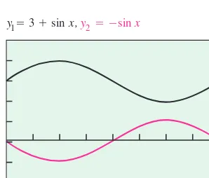
EXAMPLE 7
Applying Corollary 3
Find the function
f
x
whose derivative is sin
x
and whose graph passes through the
point
0, 2
.
SOLUTION
Since
f
has the same derivative as
g
(
x
)
– cos
x
, we know that
f
(
x
)
– cos
x
C
, for
some constant
C
. To identify
C
, we use the condition that the graph must pass through
(0, 2). This is equivalent to saying that
f
(0)
2
cos
0
C
2
fx cos xC1
C
2
C
3.
The formula for
f
is
f
x
cos
x
3.
Now try Exercise 35.In Example 7 we were given a derivative and asked to find a function with that
deriva-tive. This type of function is so important that it has a name.
DEFINITION
Antiderivative
Section 4.2 Mean Value Theorem 201
We know that if
f
has one antiderivative
F
then it has infinitely many antiderivatives,
each differing from
F
by a constant. Corollary 3 says these are all there are. In
Exam-ple 7, we found the particular antiderivative of sin
x
whose graph passed through the
point
0, 2
.
EXAMPLE 8
Finding Velocity and Position
Find the velocity and position functions of a body falling freely from a height of 0
me-ters under each of the following sets of conditions:
(a)
The acceleration is 9.8 m
sec
2and the body falls from rest.
(b)
The acceleration is 9.8 m
sec
2and the body is propelled downward with an initial
velocity of 1 m
sec.
SOLUTION