Regularization, Uncertainty Estimation and Out of Distribution Detection in Convolutional Neural Networks

(1)

Detection in Convolutional Neural Networks

Ujwal Karthik Krothapalli

Dissertation submitted to the Faculty of the Virginia Polytechnic Institute and State University in partial fulfillment of the requirements for the degree of

Doctor of Philosophy in

Computer Engineering

A. Lynn Abbott, Chair Pinar Acar Creed Jones III

Haibo Zeng Yunhui Zhu

August 13, 2020 Blacksburg, Virginia

Keywords: Regularization, Uncertainty Estimation, Classifier, Convolutional Neural Network

(2)

Regularization, Uncertainty Estimation and Out of Distribution

De-tection in Convolutional Neural Networks

(ABSTRACT)

(3)

(4)

Regularization, Uncertainty Estimation and Out of Distribution

De-tection in Convolutional Neural Networks

(GENERAL AUDIENCE ABSTRACT)

(5)

(6)

Dedication

To my parents.

(7)

I would like to express my gratitude to numerous people for helping me throughout this insightful and long journey and would like to mention a few of them.

I am forever indebted to my advisor, Dr. A. Lynn Abbott. Dr. Abbott welcomed me to his lab in 2013 and has remained a source of guidance throughout the completion of my program. His expertise, insight, and patience have helped me become the researcher that I am today. I am very thankful to my committee members, Dr. Haibo Zeng, Dr. Yunhui Zhu, Dr. Pinar Acar and Dr. Creed Jones III for their insightful comments and questions.

I would like to thank my current and past fellow lab members, especially Xiaolong Li for all the feedback, questions, and comments.

My parents, family and friends have always supported my relentless academic ambitions and encouraged me to pursue my passion in machine learning. I am forever grateful to my wonderful brother Gautam. A very special thank you to my late grandparents. Many thanks to my uncle Dr. Venkat Mummalaneni, Aunt Shobha and Aunt Lakshmi for their constant support and encouragement. I would like to thank my cousins Dr. Simha Mummalaneni and Dr. Vaishnavi Gummadi for setting a very high bar and my cousins Vaibhav and Vikram for their support and advice throughout the years.

I would like to express my gratitude for all the support and proofreading help I received from Boyce Lacy Burnett over the past year.

(8)

I was supported throughout my program by VTTI through many projects, and am espe-cially thankful to Andy Petersen for the wonderful opportunities he provided at VTTI. I have spent all my summers since 2013 working on various projects and pushing the compute infrastructure limits at VTTI. I am thankful to Bill F., Brian L., Clark G., Calvin W. and Zeb B. for their advice, friendship and support over the years at VTTI.

(9)

List of Figures xii

List of Tables xxiv

1 Introduction 1

1.1 Background . . . 4

1.1.1 Regularization . . . 4

1.1.2 Adaptive Label Smoothing. . . 7

1.2 Challenges . . . 10

1.3 Contributions . . . 10

1.4 Outline . . . 11

2 Overview 13 2.1 Deep Learning . . . 13

2.1.1 Neurons, Perceptrons and Multi-Layer Perceptrons . . . 13

2.1.2 Convolutional Neural Networks . . . 16

3 CopyPaste 19 3.1 Datasets . . . 19

(10)

3.2 Approach . . . 20

3.3 Contributions . . . 22

3.4 Related Work . . . 23

3.4.1 Classic Data Augmentation . . . 23

3.4.2 Random Noise . . . 24

3.4.3 Mixed Sample. . . 24

3.4.4 AutoAugment . . . 25

3.5 Object and Context based Data Augmentation . . . 25

3.6 Experiments . . . 27

3.6.1 ImageNet Classification . . . 28

3.6.2 Object Detection using Pretrained Model . . . 30

3.6.3 Qualitative results . . . 32

3.7 Conclusion. . . 33

4 Adaptive Label Smoothing 39 4.1 Related Work . . . 39

4.2 Method . . . 43

4.3.1 Datasets . . . 45

4.4 Experimental setup . . . 49

(11)

4.4.2 Hardware and software . . . 50

4.4.3 Runtimes . . . 50

4.4.4 Classification and calibration . . . 56

4.4.5 Transfer learning for object detection . . . 56

4.4.6 Ablation studies . . . 58

5 Out of Distribution Detection 61 5.1 Related Work . . . 61

5.2 Method . . . 62

5.4 Results. . . 77

6 Conclusions 93

Bibliography 96

(12)

List of Figures

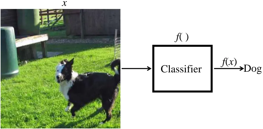
1.1 The general idea of a classifier, x is the input to a learned function f which

outputs a class label. Future discussions of classifiers in this dissertation will

refer to a CNN (f) that takes an input color image (x) and outputs a class

label. . . 2

1.2 LeNet-5 [40], a CNN used for high accuracy digit recognition. Yellow colored

layers are convolutional layers, red colored layers are max-pooling layers and

teal colored layers are fully connected layers. The layers that are not directly

connected to input and output (last layer in this figure) are called hidden

layers. The output layer is shown in magenta. Figure plotted using the

implementation of [31]. . . 4

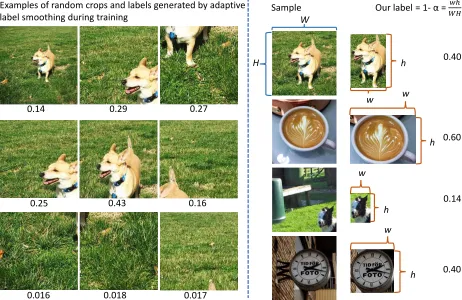
1.4 Random crops of images are often used when training classification CNNs to

help mitigate size, position and scale bias (left half of figure). Unfortunately,

some of these crops miss the object as they do not have any object location

information. Traditional hard label and smooth label approaches do not

ac-count for the proportion of the object being classified and use a fixed label of

‘1’ or ‘0.9’ in the case of label smoothing. Our approach (right half) smooths

the hard labels by taking into account the objectness measure to compute an

adaptive smoothing factor. The objectness is computed using bounding box

information as shown above. Our approach helps generate accurate labels

during training and penalizes low-entropy (high-confidence) predictions for

context-only images (the main object is completely or mostly absent). . . . 7

(13)

sents the theme of the work being pursued. . . 12

2.1 A simple neuron. . . 14

2.2 A simple perceptron. . . 15

2.3 LeNet-5, a CNN used for high accuracy digit recognition [39]. . . 17

3.1 In a classification approach, the location of the object is not accounted for while training and the expected outputs (post training) for all the 3 variations of the image should indicate Dog. The CNN has to learn to localize the pertinent object (dog in this case) and produce an output indicating the presence of the object. . . 20

3.2 Our method uses bounding box information to paste objects belonging to the same class in a given image. The red bounding box is an example of bounding box annotation and the rest of the image is considered context. The green bounding box shows the object that has been pasted from another image of the same class if bounding boxes are available. The bottom two rows are sample images generated on the fly by our approach. The labels of images in the second row (left to right) are, ‘Goldfish’, ‘Cauldron’, and ‘Alligator lizard’. The labels of images in the third row (left to right) are, ‘Tench’, ‘Snow leopard’, and ‘Robin’. . . 21

(14)

3.3 We show the differences in recent augmentation methods and the

correspond-ing labels for images generated uscorrespond-ing the different approaches. Because

Cut-Mix and RICAP have no localization information, they are more likely to

assign the wrong label to a given crop (red bordered images indicate wrong

labels and green bordered images indicate the correct labels), whereas our

approach generates correct labels all the time. ImageNet column shows the

standard images from the dataset without any augmentation so the labels are

not changed during training like the other methods. (Note: The border colors

are purely for illustrative purposes. The CNN does NOT receive the samples

with the colored borders.) . . . 34

3.4 We use a compute node that is different from our main GPU node to handle

the tremendous compute imposed by modifying the train set on the fly. The

gaps in between the high CPU use show the times during which we utilize

clean ImageNet samples. . . 35

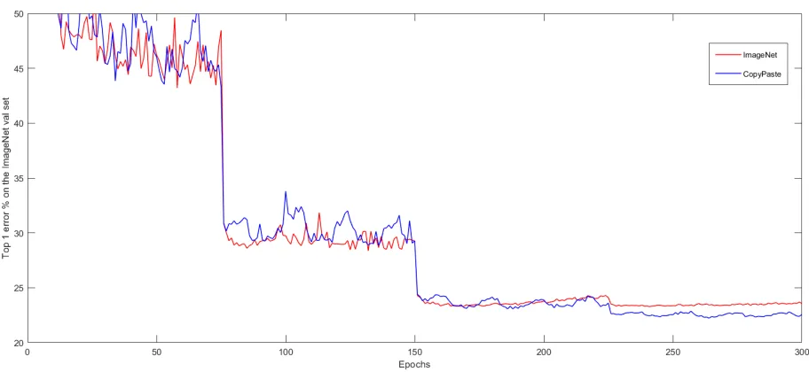
3.5 We plot the validation error during the training of the baseline approach as

well as our approach . . . 35

3.6 We plot the last lowest error (last good performance) during the course of

training the baseline model as well as our approach . . . 36

3.7 Qualitative results using class activation maps to show the most pertinent

regions used by each method to make the prediction. . . 36

3.8 More qualitative results using class activation maps to show the most

perti-nent regions used by each method to make the prediction. . . 37

(15)

regions used by each method to make the prediction. Our approach also

helps CutMix and RICAP localize the pertinent objects better. . . 38

4.1 Hard-label and label-smoothing based approaches (top half of the figure) do

not take into account the proportion of the object being classified. Our

ap-proach (bottom half) weights soft labels using the objectness measure to

com-pute an adaptive smoothing factor. . . 42

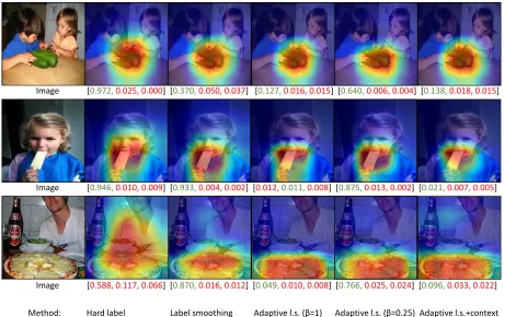
4.2 Examples of class activation maps (CAMs). These were obtained using the

implementation of [6]. Two columns on the left show results for baseline CNNs

using hard labels and standard label smoothing. Our approach,adaptivelabel

smoothing (“adaptive l.s.”), is illustrated in the three columns on the right.

Our technique produces high-entropy predictions and shows an improved

lo-calization performance. The values under each CAM represent the top three

probabilities, with green indicating the pertinent class and red indicating an

incorrect prediction. . . 46

implementation of [6]. The second and third columns from the left show

results for baseline CNNs using hard labels and standard label smoothing.

Our approach, adaptive label smoothing (‘Adaptive l.s’), is illustrated in the

three rightmost columns. Our technique produces high-entropy predictions

and shows an improved localization performance. The values under each CAM

represent the top three probabilities, with green indicating the pertinent class

and red indicating an incorrect prediction. . . 47

(16)

implementation of [6]. The second and third columns from the left show

results for baseline CNNs using hard labels and standard label smoothing.

Our approach, adaptive label smoothing (‘Adaptive l.s’), is illustrated in the

three rightmost columns. Our technique produces high-entropy predictions

and shows an improved localization performance. The values under each CAM

represent the top three probabilities, with green indicating the pertinent class

and red indicating an incorrect prediction. . . 48

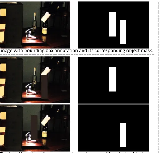
4.5 The first row of images in the left half of the figure are an example of the

Im-ageNet dataset (N=0.474M) that have bounding box annotations. We match

the images from the training set of ImageNet-1K dataset with the

correspond-ing ‘.xml’ files included in the ImageNet object detection dataset. We then

create object masks for each of the images. When applying any scaling and

cropping operation to training samples, we apply the same transformation to

the corresponding object masks as well. By counting the number of white

pix-els, we can determine the object proportion post transformation. We describe

the two other approaches in the figure, the ‘mask’ version of our approach has

a single object (for images with multiple bounding box annotations) and this

version has 0.528M samples. Our approach helps generate accurate labels

during training and penalizes low-entropy (high-confidence) predictions for

context-only images like the example on the right half of the figure. . . 51

(17)

the highest number of images in a given class is ‘1349’ and the lowest count

is ‘190’. The distribution in this case is not as skewed as the OpenImages

(bottom half) dataset. About 60 classes in our subset of the OpenImages

dataset account for half the dataset. The maximum and minimum counts are

55K and 28K respectively. . . 53

4.7 Reliability diagrams help understand the calibration performance [12, 54] of

classifiers. We compute ECE1 using the implementation of [71] on the

vali-dation set of ImageNet. The deviation from the dashed line (shown in gray),

weighted by the histogram of confidence values, is equal to Expected

Cali-bration Error [71]. The top half of the figure shows classifiers trained using

the same dataset (N=0.528M), but with different values of β. The leftmost

reliability diagram is the classic hard label setting and the rightmost

relia-bility diagram is the adaptive label setting. The bottom half of the figure

compares classifiers trained on the complete ImageNet (leftmost) with 3

clas-sifiers trained on the subset of ImageNet with bounding box labels using

different values of the α hyperparameter. . . 57

5.1 Confidence values (maximum value of the predicted output) of 50K

ImageNet-1K and 50K OImageNet-ImageNet-1K validation images plotted as a histogram with 32

equispaced bins for the hard label case. Clearly, there is no distinct way to

threshold the different distributions as they severely overlap with one another. 63

(18)

equispaced bins for the standard uniform label smoothing case. The

separa-tion is better than the hard label case, but there is plenty of overlap. . . 64

equispaced bins for our adaptive label smoothing method. The separation

is better than the hard label and label smoothing cases, as we produce low

confidence scores for a much larger number of out of distribution samples. . 65

equispaced bins for our adaptive label smoothing method with β = 0.75. . . 66

equispaced bins for our adaptive label smoothing method with β = 0.25. . . 67

equispaced bins for our adaptive label smoothing method with 5 percent of

training samples are context only and 5 percent of samples are from 500

classes of OImageNet training set. . . 68

(19)

1K and 50K OImageNet-1K validation images plotted as a histogram with 32

equispaced bins for our adaptive label smoothing method with 5 percent of

training samples are context only and 5 percent of samples are from 1000

classes of OImageNet training set. . . 69

5.8 Entropy values of 50K ImageNet-1K and 50K OImageNet-1K validation

im-ages plotted as a histogram with 32 equispaced bins for the hard label case.

Clearly, there is no distinct way to threshold the different distributions as

they severely overlap with one another. . . 70

im-ages plotted as a histogram with 32 equispaced bins for the standard uniform

label smoothing case. The separation is better than the hard label case, but

there is plenty of overlap. . . 71

im-ages plotted as a histogram with 32 equispaced bins for our adaptive label

smoothing method. The separation is better than the hard label and label

smoothing cases, as we produce low Entropy scores for a much larger number

of out of distribution samples. . . 72

smoothing method with β = 0.75. . . 73

smoothing method with β = 0.25. . . 74

(20)

smoothing method with 5 percent of training samples are context only and 5

percent of samples are from 500 classes of OImageNet training set. . . 75

smoothing method with 5 percent of training samples are context only and 5

percent of samples are from 1000 classes of OImageNet training set. . . 76

equispaced bins for our adaptive label smoothing method withβ = 0.75, 5

percent of training samples are context only and 0 percent of samples are

from 1000 classes of OImageNet training set. . . 78

smoothing method withβ = 0.75, 5 percent of training samples are context

only and 0 percent of samples are from 1000 classes of OImageNet training

set. . . 79

(21)

ages plotted as a histogram with 32 equispaced bins for our adaptive label

set. . . 81

set. . . 83

only and 5 percent of samples are from 500 classes of OImageNet training set. 85

(22)

set. . . 87

set. . . 89

(23)

1K and 50K OImageNet-1K validation images plotted as a histogram with 32

set. . . 91

(24)

List of Tables

3.1 ImageNet classification accuracies using ResNet-50 architecture. ‘*’ denotes

results reported in their paper. . . 28

3.2 ImageNet cross entropies and gaps using ResNet-50 architecture. . . 29

3.3 Object detection mean average precision values using ResNet-50 backbone

and Faster-RCNN. We report the best out of last 3 epochs for all methods. 31

and Faster-RCNN for small objects in COCO. We report the best out of last

2 epochs for all methods. . . 32

4.1 Confidence and accuracy metrics on the validation set of ImageNet with all

the objects removed using bounding box annotation provided by [8]. . . 44

4.2 Classification and calibration results with ImageNet. For a detailed

explana-tion of the metrics please refer to the ‘Experimental setup’ secexplana-tion. ‘A.conf’,

‘O.conf’ and ’U.conf’ refer to average confidence, overconfidence, and

under-confidence scores. We provide ECE values for 100 bins and 15 bins mean

scores along with their standard deviation (std). . . 52

(25)

nation of the metrics please refer to the ‘Experimental setup’ section. ‘A.conf’,

‘O.conf’ and ’U.conf’ refer to average confidence, overconfidence, and

under-confidence scores. We provide ECE values for 100 bins and 15 bins mean

scores along with their standard deviation (std). . . 54

4.4 Fine-tuning on MS-COCO using FRCNN for object detection. For a detailed

explanation of the results please refer to the ‘Experimental setup’ section.

AP refers to average precision and AR refers to average recall at the specified

Intersection over union (IoU) level. We also provide AP values for small,

medium, and large objects using ‘S’, ‘M’, and ‘L’ respectively. . . 55

(26)

Chapter 1

Introduction

Categories are ubiquitous in almost all datasets. Classification can be defined as the problem of recognizing the category of a given observation. Classification is a well studied statistical problem with a significant amount of progress made in the past decade. It is the basic building block of many applications pertaining to the areas of Computer Vision, Speech Recognition and Natural Language Processing. To train a good classifier, usually a large number of diverse (independent and identically distributed) samples are needed and it is important to prevent the classifier from overfitting to the training samples.

The task of classifying/identifying objects in images is very easy for humans with good vision capabilities however, machines have a diﬀicult problem of relying on millions of pixel values to produce a probability distribution for the same classification task. The human visual cor-tex is very advanced compared to the state of the art artificial neural networks. The latest advances in the field of deep neural networks (DNNs) show that surpassing human capabil-ity when it comes to certain computer vision tasks is possible. Deep convolutional neural networks (CNNs) have been used for solving various computer vision problems, especially image classification [40] with tremendous success using large datasets since 2013 [32,60]. By pairing the hierarchical approach of DNNs with cross-correlation operations, CNNs can learn complex representations required for classification. Overfitting in this context refers to the phenomenon of simple memorization of the input samples by the CNN (model) rather than reasoning about the salient features of the samples so the classifier may not generalize to

(27)

unseen samples. With ever increasing size of neural networks [25, 61], there is a need for vast amount of labeled data [47] and better generalization, as simply increasing the number of parameters in a neural network will often lead to overfitting of the training data. Model capacity is defined as the ability of a model to learn complex tasks, and a larger model usually will be able to approximate and learn to represent more complex data distributions. Training data and an objective function are some of the first design choices that one must consider when training a classifier. Modern day CNNs have a large number of parameters and often suffer from many problems when deployed in the real world. Lack of diverse train-ing data is one of the problems. A popular class of methods used to improve the diversity of training data is known as data augmentation.

f

( )

x

Dog

f

(

x

)

Classifier

Figure 1.1: The general idea of a classiﬁer, x is the input to a learned function f which outputs a class label. Future discussions of classiﬁers in this dissertation will refer to a CNN (f) that takes an input color image (x) and outputs a class label.

(28)

3

the training dataset. The learnt parameters of a classifier are often referred to as weights. In the case of CNNs, an input layer is the part of a CNN that takes the raw input and outputs a representation of the input. In the case of images, the input layer usually consists of simple image operations like edge detectors that have been learnt.

The output layer of a classification CNN is usually a vector whose length is equal to the number of classes present in the training data. Any layer that is sandwiched between an input layer and an output layer of a neural network is referred to as a hidden layer, as shown in figure 1.2. To solve complex problems, a higher number of hidden layers are used as this allows the neural network to approximate complex distributions of data. The ability of a neural network to learn nuanced differences in the data is referred to as the network’s expressive power. The higher the number of hidden layers the higher the expressive power of the classifier. In the case of a simple square RGB image with each side equal to 224 pixels and each pixel having an intensity of 0 to 255, the number of possible images is extremely large, 2563×224×224 _{to be precise. The classification CNNs in this dissertation are trained to}

(29)

132

6 28

16 10

1120

184

10

SOFT

Figure 1.2: LeNet-5 [40], a CNN used for high accuracy digit recognition. Yellow colored layers are convolutional layers, red colored layers are max-pooling layers and teal colored layers are fully connected layers. The layers that are not directly connected to input and output (last layer in this ﬁgure) are called hidden layers. The output layer is shown in magenta. Figure plotted using the implementation of [31].

1.1

Background

1.1.1

Regularization

(30)

gen-1.1. Background 5

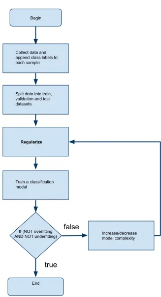
eralization performance when a finite number of training samples are present. Since 2013, numerous data augmentation and regularization methods have been proposed and are a part of standard training procedure for CNNs [28, 32, 63,67]. In order to prevent simple memo-rization of the training data (over-fitting) and to constrain the complexity of the classifier, strong regularization is needed. Figure 1.3 shows a flowchart of the steps typically followed in the process of training a classifier. Data augmentation has proven to improve classifier performance at no additional computational cost at test time and is a very active area of research. Categorical labels are used for training CNNs. These labels indicate which class (category) of object is present in a given image. These labels do not have any information

on the location of the object in a given image.

The goal of this work is to show that regularization of existing classifiers can also be done using labels that are not only categorical but also with labels that localize the relevant object in a given image. We explore the idea of using the labels that localize the object to train better classifiers and object detectors as this is a very active area of research [32, 60, 69, 74].

Early stopping of the training scheme to prevent over-fitting, dropout (dropping hidden layer activations randomly while training) and weight decay (penalizing the norm of the model’s parameters) fall under the umbrella of explicit regularization methods, whereas image operations such as randomly cropping a subregion, randomly changing the aspect ratio and randomly adding a positive or negative value to the pixel intensities of an image fall under the umbrella of data augmentation methods. Some of the data augmentation methods can be applied in the feature (hidden) space and these methods are then closer to explicit regularization methods (for example, [63]).

(31)

However, when some of the new data augmentation methods are used, the classifier (model) learns shape specific features of the objects rather than focusing on just their texture. This is one of the several motivating factors for our work.

Randomly dropping hidden layer activations as proposed in dropout [63] and randomly dropping part of input pixels as [13, 20, 62, 79] have improved the ability of CNNs to localize and classify objects in a given image. All the above mentioned data augmentation methods have a regularization effect and most of the methods can be used in conjunction with one another after empirical validation, as the theory behind such methods is not fully understood.

(32)

1.1. Background 7

1.1.2

Adaptive Label Smoothing

Examples of random crops and labels generated by adaptive label smoothing during training

H

Sample Our label = 1-α= _𝑊𝐻𝑤ℎ

0.40 0.60 0.14 0.40 W w h w h w h w h 0.27 0.29 0.14 0.16 0.43 0.25 0.017 0.018 0.016

Figure 1.4: Random crops of images are often used when training classification CNNs to help mitigate size, position and scale bias (left half of figure). Unfortunately, some of these crops miss the object as they do not have any object location information. Traditional hard label and smooth label approaches do not account for the proportion of the object being classified and use a fixed label of ‘1’ or ‘0.9’ in the case of label smoothing. Our approach (right half) smooths the hard labels by taking into account the objectness measure to compute an

adaptive smoothing factor. The objectness is computed using bounding box information as shown above. Our approach helps generate accurate labels during training and penalizes low-entropy (high-conﬁdence) predictions for context-only images (the main object is completely or mostly absent).

(33)

to the gap in accuracy and confidence of a classifier. There is a growing demand for labeled data [47] to improve generalization performance, as increasing the number of parameters in a neural network [64, 76] will often lead to overfitting of training data, and obtaining an exponentially large labeled dataset is very expensive. Safely deploying deep learning based models has become an immediate challenge [2] as CNNs are being used in a variety of applications. As a community, apart from obtaining high accuracies, we also need to provide reliable uncertainty measures of CNNs. By having reliable confidence measures, we can improve precision (the number of correct predictions divided by all the predictions pertaining to a class) by not acting with certainty when uncertain predictions are produced, as in the case of safety-critical systems.

(34)

1.1. Background 9

improvement in learning speed and generalization; in contrast, hard targets tend to increase the values of the logits and produce overconfident predictions [50, 66]. We illustrate the different labels used by CNNs in figure 1.4.

Object detection [21] is a well-studied problem and most approaches need bounding box information during training. Recently, [16] proposed using novel synthetic images to im-prove the object detection performance by augmenting training data using object location information. However, classification CNNs have not exploited bounding box information to regularize CNNs on large datasets to our knowledge. The concept of ‘Objectness‘ was first introduced by [1], and the role of objectness has been studied extensively since then. Quantifying the likelihood an image window contains an object belonging to any class makes the measure class agnostic.

(35)

1.2

Challenges

There are many challenges that plague modern day CNNs. This dissertation brings to light the following problems.

1) Augmentation methods used for images used to train classification CNNs do not distin-guish object pixels from context pixels. This inattention (to object pixels) introduces context dependence (prediction the class of an image using context rather than object).

2) Reliability: CNNs are overconfident and fail to provide confidence measures that are reliable.

3) Out of distribution detection: CNNs produce highly confident wrong predictions even on images belonging to classes that were not used during training. This is problematic in the real world where many novel classes exist.

1.3

Contributions

We develop novel and intuitive solutions to the above challenges. The major contributions are as follows:

(36)

1.4. Outline 11

2) A classifier whose confidence is grounded in object size. We develop a novel way to force a CNN to produce confidence values that correspond to the relative object proportion in a given image. We show that this approach improves localization performance and produces more reliable predictions.

3) Out of object detection by generating high entropy/low confidence predictions on un-seen data. Using this approach we can neglect predictions whose confidence is below a certain threshold, thereby improving precision.

1.4

Outline

This dissertation is organized as follows.

1) Chapter 1: Provides an introduction to this dissertation.

2) Chapter 2: Provides an overview and history of CNNs.

3) Chapter 3: Presents our regularization approach CopyPaste, that leverages object location information during training.

4) Chapter 4: Presents our work, Adaptive Label Smoothing.

5) Chapter 5: Presents our work on Out of Distribution Detection.

(37)

Begin

Collect data and append class labels to each sample

Regularize

Train a classification model

If (NOT overfitting AND NOT underfitting)

false

true

Split data into train, validation and test datasets

End

Increase/decrease model complexity

(38)

Chapter 2

Overview

This chapter of dissertation will introduce the history and theory behind deep learning in a supervised setting and provide motivation for this work. A detailed description of related work is also provided.

2.1

Deep Learning

The subsections will describe the history behind modern Convolutional Neural Networks (CNNs) beginning with the idea of a Neuron and then Multi-Layer Perceptrons (MLPs).

2.1.1

Neurons, Perceptrons and Multi-Layer Perceptrons

The idea of an artificial neuron can be traced to 1943 when Warren McCulloch and Walter Pitts proposed the McCulloch-–Pitts neuron. The authors presented a mathematical basis to model an artificial neuron with inputs and a binary output. The McCulloch-–Pitts neuron was modeled to accept multiple binary inputs xi which were multiplied by the weights wi (represented between -1 and +1). The valueswixi were then summed to compute a weighted sum S. The neuron is said to have fired when the weighted sum S was greater than a threshold T [48]. The threshold T is also called an activation function. The neuron was able to perform logical operations like AND, OR and NOT by using appropriate thresholds

(39)

and inputs. The activation function of the McCulloch-–Pitts neuron is a step function or a Heaviside function. Mathematically, the weighted sum S is computed using the equation:

S= n ∑

i=1

wixi (2.1)

The output y of the McCulloch-–Pitts neuron is a binary variable. The output can be 0 or 1 and is computed using the equation:

y=f(s) =       

1 for s≥T 0 for s < T

(2.2)

Figure 2.1: A simple neuron.

(40)

2.1. Deep Learning 15

mathematical representation to:

S = n ∑

i=1

wixi+b (2.3)

The weight updates can be represented as:

∆wij =ηyjxi (2.4)

Learning the perceptron is made possible by using the wij which is referred to the weight update. The weight update is equal to the product of learning rate of the perceptron η, the inputs xi and the output yj.

Figure 2.2: A simple perceptron.

Limitation of the perceptron was the input data had to be linearly separable. Apart from simple logic gates, non-linearly separable cases like XOR could not be solved using the perceptron model.

(41)

The architecture of FFNNs is simple, a layer of perceptrons feeds the next layer and this process connects the input layer with that of the output with multiple hidden layers. To train FFNNs, backpropagation is employed, this method takes advantage of the chain-rule to propagate the updates. The weights of the network are updated based on the error measured at the output layer and propagated all the way back to the input layer in a layer by layer fashion. When backpropagation is performed in an iterative fashion over all the samples in a training set, the process is called gradient descent.

2.1.2

Convolutional Neural Networks

The Multi-Layer Perceptrons (MLPs) were extended to work with images. In 1980 Kunihiko Fukushima proposed the Neocognitron. By using a combination of simple and complex cells the Neocognitron was able to provide translational invariance for recognition tasks [18].

The term Convolutional Neural Network (CNN) was popularized by LeCun et al.in 1990. It was used to classify handwritten digits with an accuracy of 99% [41]. The model was called ‘LeNet’, the network was able to classify handwritten digits with variance in position, scale

and appearance.

CNNs evolved with the advent of parallel computing resources like GPUs and the availability of labeled data. In 2012 a CNN called “AlexNet” by Krizhevsky et al. formally brought the methods to a wide audience by competing in the 2012 “ImageNet” challenge and surpassing all classic computer vision baselines. The AlexNet enabled modern CNNs which are being used every day by consumers all over the world.

(42)

2.1. Deep Learning 17

132

6 28

16 10

1120

184

10

SOFT

Figure 2.3: LeNet-5, a CNN used for high accuracy digit recognition [39].

layers.

Convolution in this case is an operation involving two functions like, f which is the input and g the kernel. The result of convolution can be represented by h. The function h can be computed by integrating the overlap of f and g. In a signal processing approach this is represented as:

h(t) = (f∗g)(t) = ∫ _∞

−∞f(δt)g(t−δt) dδt (2.5)

(43)

per-formed over two dimensions in the case of images. The convolution operation with kernel K over imageI is progressed by the sliding window method. The kernelK is slid incrementally over the input image producing a feature mapH. Mathematically:

H(i, j) = (I∗K)(i, j) =∑ m

∑

n

I(m, n)K(i−m, j−n). (2.6)

To suppress the unimportant regions in the feature maps, a pooling operation layer is em-ployed in the network, this layer also reduces the image dimensions. The common types of pooling layers are Max pool and Average pool. This layer adds some spatial invariance to the network as well. Simply composing a network with multiple convolutional and pooling layers is not enough, to inject non-linearity, a transfer function is employed. A rectified linear unit or (ReLU) is one of the most commonly used activation or transfer functions. The output of ReLU differs from that the sigmoid function as ReLU is not limited between 0 and 1. The lower bound of ReLU and sigmoid functions is 0 and their outputs are always positive. The ReLU’s upper bound is the input itself x.

(44)

Chapter 3

CopyPaste

This chapter is dedicated to our regularization technique called, CopyPaste.

3.1

Datasets

We evaluate our classification approach on the ImageNet-1K dataset [60]. The dataset con-sists of about 1.28M million training images and 50 thousand validation images with 1000 categories (classes). In addition to class labels, about 38 percent of the training images have 2 dimensional coordinates specifying a rectangular bounding box to enclose the pertaining object. We use the bounding box annotations for these images in our approach for classifi-cation. ImageNet pre-trained models are used for many other visual recognition tasks like object recognition. And to evaluate the object detection performance, we use the MS-COCO dataset [44]. It has 80 object classes for object detection and there are about 118 thousand images for training and 5 thousand images for validation. We also evaluate on Pascal VOC 2007 and 2012 [17] trainval data of about 33 thousand images and 20 categories. The object detection models are then validated on VOC 2007 test data consisting of about 5 thousand images.

(45)

x

x1

x2

f( )

Dog

f(x)

Classifier

Figure 3.1: In a classiﬁcation approach, the location of the object is not accounted for while training and the expected outputs (post training) for all the 3 variations of the image should indicate Dog. The CNN has to learn to localize the pertinent object (dog in this case) and produce an output indicating the presence of the object.

3.2

Approach

(46)

3.2. Approach 21

+

=

Figure 3.2: Our method uses bounding box information to paste objects belonging to the same class in a given image. The red bounding box is an example of bounding box annotation and the rest of the image is considered context. The green bounding box shows the object that has been pasted from another image of the same class if bounding boxes are available. The bottom two rows are sample images generated on the ﬂy by our approach. The labels of images in the second row (left to right) are, ‘Goldﬁsh’, ‘Cauldron’, and ‘Alligator lizard’. The labels of images in the third row (left to right) are, ‘Tench’, ‘Snow leopard’, and ‘Robin’.

all strict classification problems.

(47)

However, even the most recent approaches in the area of classification do not incorporate bounding box information of the objects present in them. We use bounding box information when available during training of our classifier by identifying the class of a given image and pasting an object of the same class on it. Figure 4.1 shows our approach on some of the training samples. The bottom two rows are samples generated by our approach. We use objects and paste them anywhere in a given image, the intuition being that objects of the same class share similar context. Our approach is label preserving because we do not have to change the labels of our transformed images. We can generate infinitely many combinations of objects and context at different scales and locations. This is a powerful way to regularize CNNs. Our approach also improves classification performance, small object detection and localization in general.

Figure 3.3 shows the differences between our method and the other recent approaches. Cut-Mix and RICAP change the label of an image based on the proportion of pixels represented by each class and the ‘mixing’ of samples is random. Our method is label preserving (correct labels are passed to the classifier during training) as opposed to CutMix and RICAP which use random crops to mix samples from different classes. Incorrect labels hurt the training of CNNs, and CutMix and RICAP often use context crops instead of object crops, but supply the label of the object in the image to the CNN. We argue that this inconsistency can lead to context dependence as the authors of RICAP [69] point out in their work.

3.3

Contributions

(48)

3.4. Related Work 23

• A novel way to use bounding box annotations for data augmentation of classification CNNs with complete control over the augmented object location and scale.

• We are able to produce a quantifiable improvement in classification accuracy of the standard CNN baseline on ImageNet dataset [60].

• We outperform standard CNN baseline on MS-COCO [44] object detection.

• We combine our approach with other data augmentation methods to realize further improvements in performance of the other methods.

3.4

Related Work

We propose a novel data augmentation technique and show how it is related to recent devel-opments in this area.

3.4.1

Classic Data Augmentation

(49)

training. However, they are not suﬀicient to reduce the effect of over-fitting on their own, as newer CNN architectures can have almost 100 million parameters and billions of floating point operations.

3.4.2

Random Noise

The random noise class of data augmentation methods [13, 79] work by masking random regions of an input image with zeros. These methods may accidentally erase the pertaining object in a given image, forcing the CNN to rely purely on context at times to make a prediction. Relying on context only is not an eﬀicient way to train neural networks. This approach can also be applied to the inputs of hidden layers (also known as feature space) as well. The authors of DropBlock [20] have used this technique (applying random noise to the feature space) to obtain better generalization. The authors of [7, 62]use random noise based methods to obtain better localization characteristics.

3.4.3

Mixed Sample

In the case of classification CNNs, the ground truth/labels are represented by a one-hot representation of class probabilities. These labels consist of 0s and 1s, with a single 1 indicating the pertinent class in a given label vector. The latest work in the area of data augmentation involves using samples from different classes and changing the expected output of the CNN to output a probability distribution based on the number of pixels/intensity of pixels represented by each class.

(50)

3.5. Object and Context based Data Augmentation 25

as opposed to cut-paste methods like RICAP and CutMix.

Having soft labels (label values in between 0 and 1) is an advantage while training CNNs as the probabilities output by a CNN are never perfect0sand1sand the CNNs usually produce overconfident results even when their predictions are wrong. The authors of CutMix and RICAP [69, 74] also use soft labels in their approach. In our case since the samples being mixed are from the same class, we do not have to change the label. This allows for easy integration with CutMix and RICAP [69, 74] as well.

3.4.4

AutoAugment

In order to learn the best augmentation strategy dynamically during training, the authors of AutoAugment [10] use reinforcement learning to learn the best combination of existing data augmentation methods.

3.5

Object and Context based Data Augmentation

In this section, we describe the data augmentation methods of interest in mathematical detail.

Consider D = ⟨(xi, zi)⟩Ni=1 to be a dataset consisting of N independent and identically

distributed real-world images belonging to K different classes. Let _X represent the set of images, and letY denote the set of ground-truth class labels. Sampleiconsists of the image xi ∈ X along with its corresponding label zi ∈ Y = {1,2, ..., K}. Let fθ represent the CNN classifier with model parameters θ. The predicted class isyˆi = argmaxy∈Y pˆi,y, where ˆ

(51)

In the case of Mixup with two samples,(xi, zi)∼Dand (xj, zj)∼D, the transformed image and label pair (˜x,z)˜ are computed as,

˜

x=λxi+ (1−λ)xj (3.1)

˜

z =λzi + (1−λ)zj (3.2)

where λ∼Beta(γ, γ) and γ is a hyperparameter set to 0.3 by default.

In the case of RICAP with 4 samples,(x1, z1)∼D,(x2, z2)∼D,(x3, z3)∼Dand(x4, z4)∼

D. The authors patch the upper left, upper right, lower left, and lower right regions of the

four images to generate a new sample.

LetW and H denote the proportions of the original image.

To crop the four images k following the sizes (wk, hk), the authors generate the coordinates of the upper left corners of the cropped areas randomly.

The ratio Wi is computed proportional to the area occupied by each patch from one of the four images. The label z˜is computed as:

˜

z = ∑

k∈{1,2,3,4}

Wkzk (3.3)

where Wk= wkhk

W H (3.4)

In the case of CutMix with two samples, the label z˜is computed as:

˜

z = ∑ k∈{1,2}

(52)

3.6. Experiments 27

where Wk= wkhk

W H (3.6)

Our method is called CopyPaste and it is used to generate a new training sample (˜x,z)˜ by combining two training samples(xi, zi) and (xj, zj) from the same class.

The training sample (˜x,z)˜ is used to train the model with the same label as the classes of both samples are the same. We use the 480K images from the ImageNet dataset that have bounding box annotations and the label remains unchanged.

˜

z =zi (3.7)

For implementation, we use a network storage as our approach continuously changes the proportion of original samples and CopyPaste-d samples over the course of training and is compute intense. We handle our augmentation operation using a dedicated node.

Our approach can be used without any changes to the loss function or the network architec-ture.

We use traditional data augmentation methods and scale/crop objects before pasting them on images of the same class. We believe this helps our performance when detecting small and multiple objects.

3.6

Experiments

(53)

Table 3.1: ImageNet classiﬁcation accuracies using ResNet-50 architecture. ‘*’ denotes re-sults reported in their paper.

Model # Parameters Top-1

Err (%)

Top-5 Err (%)

ResNet-50 (Baseline) 25.6 M 23.28 6.92

ResNet-50 + RICAP [69] 25.6 M 21.9 6.17

ResNet-50 + CutMix [74] 25.6 M 21.60 6.04

ResNet-50 + DropBlock* [20] 25.6 M 21.87 5.98

ResNet-50 + CutMix [74] + CopyPaste 25.6 M 21.48 5.85

ResNet-50 + RICAP [69] + CopyPaste 25.6 M 21.75 6.16

ResNet-50 + CopyPaste 25.6 M 22.23 6.376

3.6.1

ImageNet Classiﬁcation

We train our classifiers on ImageNet-1K dataset [60]. The classification CNNs in this dis-sertation are trained to detect 1000 different classes of images as the popular ImageNet [60] dataset consists of 1000 classes and is widely used by researchers to benchmark new ap-proaches for classifying data and to adapt to secondary tasks such as object detection.

The dataset consists of 1.2M training images and 50K validation images of one thousand categories. We use the usual data augmentation strategies for all methods. We train all the CNN models for 300 epochs starting with a learning rate of 0.1 and decayed by 0.1 at epochs 75, 150, and 225 using a batch size of 256 using ResNet-50 [25] architecture for all of our experiments for a fair comparison. We use the standard data augmentation used by [25, 29, 65] for all the methods. We do not use any dropout [63] but employ Batch Normalization [30] as it is a part of the standard ResNet architecture.

Results for the classification task on ImageNet are provided in table 3.1. Our approach by itself does not have the best performance as it can be considered as a special case of CutMix. However, when combined with CutMix we see the best performance 21.488%top-1 error.

(54)

dis-3.6. Experiments 29

Table 3.2: ImageNet cross entropies and gaps using ResNet-50 architecture.

Model # Parameters Cross Entropy

Training

Cross Entropy Validation

Distribution and Generalization Gap

ResNet-50 (Baseline) 25.6 M 0.685 0.965 0.280

ResNet-50 + CutMix [74] 25.6 M 2.022 0.880 -1.142

ResNet-50 + CopyPaste 25.6 M 0.755 0.904 0.149

tribution and generalization gaps of the classifiers. Heavy augmentation like MixUp during training produces samples that are unnatural compared to the distribution of unaugmented validation samples. Ideally, the distribution gap between augmented and unaugmented sam-ple distributions (augmented samsam-ples belong to a slightly different distribution compared to the unaugmented samples) can be measured by computing the mean cross entropy loss across all training samples. We compute the difference between the mean cross entropy of augmented training samples and the mean cross entropy of unaugmented validation samples thereby computing both distribution gap as well as generalization gap together 3.2. Our approach produces the lowest gap compared to the other baselines.

Our approach is called CopyPaste, but we also refer to it as CutPaste as it involves the same operation of using bounding box operation to copy or cut the object region and paste it on top of a target image belonging to the same class. We do not use additional images than the train set of ImageNet, we cross reference the images that have bounding box annotation with the images in the train set and only use those images to augment.

(55)

When copying we use the standard data augmentation operations on the object patch before pasting in on a given image. Figure 3.4 shows the compute plot of our dedicated node performing augmentation and copying the clean ImageNet samples cyclically. Figure 3.5 shows the validation error of the ImageNet dataset using standard ResNet-50 on CopyPaste-d CopyPaste-data anCopyPaste-d the clean ImageNet CopyPaste-data. StanCopyPaste-darCopyPaste-d ImageNet training starts over-fitting arounCopyPaste-d epoch 150. However, our approach continues to improve and produces a lower top 1 error rate.

Figure 3.6 shows that our model produces the lower error and is improving continuously as our last good error rate drops consistently.

3.6.2

Object Detection using Pretrained Model

We use the implementation of Faster RCNN [58] adapted to use the ResNet-50 backbone. The ResNet-50 backbone is trained with different augmentation approaches and fine-tuned on Pascal VOC 2007 and 2012 [17] trainval data. The object detection models are then validated on VOC 2007test data using the mAP measure.

We follow the fine-tuning strategy of the original methods [58]. We use the implementation of [73] to benchmark the backbones trained using different approaches. Results are provided in table3.3. Our approach obtained the best mAP (mean average precision) of the two most important baselines.

We train the models with a batch size of 8 and initial learning rate of 0.01 decayed after 5 epochs and trained for a total of 12 epochs. We report the best mAP out of the last 3 epochs for all the methods. We drop the learning rate at 8 epochs and train for 12 epochs and report the best mAP out of the last 4 epochs in table 3.4

(56)

3.6. Experiments 31

Table 3.3: Object detection mean average precision values using ResNet-50 backbone and Faster-RCNN. We report the best out of last 3 epochs for all methods.

Backbone # Parameters mAP

mAP (%)

ResNet-50 (Baseline) 25.6 M 77.63

ResNet-50 + CutMix [74] 25.6 M 77.69

ResNet-50 + CutMix [74] + CopyPaste 25.6 M 77.69

ResNet-50 + CopyPaste 25.6 M 77.90

mAP (%)

ResNet-50 + CutMix [74] 25.6 M 77.74

learning rate and train for 2 more epochs. We use a batch size of 16 and report the best numbers out of the last two epochs.

The results show that MS-COCO mAP performance of CutMix is improved when CopyPaste-d samples are useCopyPaste-d insteaCopyPaste-d of clean ImageNet samples as shown in table 3.5.

In the case of small objects, as shown in table 3.6, our approach is comparable to CutMix and provides the best improvement when a backbone trained with CutMix and CopyPaste is used.

0.50:0.95

ResNet-50 + CutMix [74] 25.6 M 31.8

(57)

Backbone # Parameters mAP 0.50:0.95 (small)

ResNet-50 + CutMix [74] 25.6 M 13.3

Table 3.6: Object detection mean average precision values using ResNet-50 backbone and Faster-RCNN for small objects in COCO. We report the best out of last 2 epochs for all methods.

In the next section, we discuss some visualizations that provide more insight into the local-ization ability of our model.

3.6.3

Qualitative results

We show qualitative results comparing various methods on ‘CopyPaste-d’ samples as well as regular samples. Our approach shows better localization characteristics, we use implementa-tion of [80] to compute the class activation maps. These maps show the most discriminating regions that the classifier relies on to make its predictions. Class activation maps (CAMs) are extremely useful in debugging CNNs as they show whether the model is simply memo-rizing the samples or learning to localize pertinent objects and classify properly. As shown in figures 3.7 and 3.8, our approach pays attention to small objects and covers a greater extent of the pertinent object(s) compared to other methods.

(58)

3.7. Conclusion 33

3.7

Conclusion

We show that bounding box annotations provided in the ImageNet dataset even for a subset of images (480k) can be used to CopyPaste using images of the same class to help improve classification and object detection performance.

Our approach however has a significant overhead and we use a network storage and separate node to augment our data on the fly.

(59)

Method: ImageNet CutMix Ours RICAP

Label: Cat 1.0 Cat 0.75, Dog 0.25 Cat 1.0 Cat 0.6, Dog 0.2, Ship 0.2, Fish 0.1

Label: Ship 1.0 Ship 0.75, Fish 0.25 Ship 1.0 Ship 0.6, Dog 0.2, Fish 0.2, Dog 0.1

Label: Fish 1.0 Fish 0.75, Ship 0.25 Fish 1.0 Fish 0.6, Ship 0.2, Dog 0.2, Cat 0.1

(60)

3.7. Conclusion 35

Figure 3.4: We use a compute node that is diﬀerent from our main GPU node to handle the tremendous compute imposed by modifying the train set on the ﬂy. The gaps in between the high CPU use show the times during which we utilize clean ImageNet samples.

(61)

Figure 3.6: We plot the last lowest error (last good performance) during the course of training the baseline model as well as our approach

Method: ImageNet Ours Ours+CutMix RICAP Ours+RICAP

(62)

3.7. Conclusion 37

Method: ImageNet Ours Ours+CutMix RICAP Ours+RICAP

(63)

Method: ImageNet Ours CutMix Ours+CutMix RICAP Ours+RICAP

(64)

Chapter 4

Adaptive Label Smoothing

The main contribution of this work is that we have developed a novel way to train clas-sification CNNs using adaptive label smoothing. To demonstrate improved classification performance with less likelihood of overconfidence, we trained 20 classifiers and evaluated them on four popular datasets.

4.1

Related Work

Bias exhibited by machine learning models can be attributed to many underlying statistics present in datasets and model architectures [5, 78] including context, object texture [19], size, shape and color in the case of images. Various approaches to mitigate bias have been proposed [3,9,19] in recent years. Our approach produces high entropy predictictions when context-only images are provided as input during inference, as we aim to learn the size of the relevant object within the image and classify it, instead of relying on context to produce a prediction.

Label smoothing was introduced by [66], and a more recent improvement is [15], correla-tions between the classes observed during training are used to provide a smooth label in an iterative fashion. This approach however has the problem of encouraging the model to make a mistake that is closer to the pertinent class. Also, using class similarity based on wordnet similarity may not always reflect image/feature similarity computed by a CNN. Knowledge

(65)

distillation [4] can be used to compute a soft label that is based on visual similarity, however this still doesn’t mitigate the problem of encouraging class confusion especially for safety-critical applications. Both adaptive regularization and knowledge distillation involve changes to the network architecture.

The authors of AlexNet [32] employed random cropping and horizontal flipping methods when they surpassed the performance of traditional machine learning approaches in 2012. Traditionally, any label preserving transformation on an input image is considered to help regularize a CNN. Randomly cropping a given image during training prevents overfitting the scale or location of the object; flipping an image improves the generalization to view points. The random noise class of data augmentation methods [13, 79] mask random regions of an input image with zeros. Random noise based methods may accidentally erase the pertinent object in a given image and force the CNN to rely purely on context to make a prediction, this contributes to label noise. The authors of DropBlock [20] have used this technique (applying random noise to feature space) to obtain better generalization. Authors of AutoAugment [10] used reinforcement learning dynamically during training to learn the best combination of existing data augmentation methods.

In contrast to augmentation based approaches that manipulate the input but not the corre-sponding label, our approach regularizes classification CNNs by computing a label based on the proportion of the object being classified in a given random crop of the training sample. The latest work in the area of data augmentation uses samples from different classes and changes expected outputs to predict a probability distribution based on the number and in-tensity of pixels represented by each class. The authors of Mixup [70,77] use alpha blending (weighted sum of pixels from two different classes), and apply blending weights to

(66)

4.1. Related Work 41

corresponding regions in the final augmented sample. The sample mixing based approaches above do not rely on object size when ‘mixing’ regions in images and computing the label. Conversely, our approach uses bounding box information to apply a smoothing factor based on the object’s size relative to the image size to produce a soft label without mixing the samples.

Calibration of CNNs is important as predictions need to be equally accurate and confident. Calibration and uncertainty estimation of predictors has been an ongoing interest to the machine learning community [12, 43, 52, 56,75]. Bayesian binning into quantiles(BBQ) [53] was proposed for binary classification and beta calibration [33] employed logistic calibration for binary classifiers. In the context of CNNs, [24] proposed a temperature scaling approach to improve calibration performance of pre-trained models. Calibration has been explored in multiple directions; popular approaches to calibrate CNNs are to transform outputs of pre-trained models using approximate bayesian inference [46], or to use a special loss function to help regularize the model [35,55] during training. Our approach is loosely related to the latter class of methods. Our work also relates to label smoothing proposed first by [66], with its applicability for many tasks explored by [55]; [72] applies dropout-like noise to the labels. Recently, [50] explored the benefits of label smoothing; apart from having a regularizing effect, label smoothing helps reduce intra-class distance between samples [50]. Another approach to calibrate CNNs was proposed by [49], using a special loss function and temperature scaling, the authors were able to obtain state-of-the-art calibration performance. Label smoothing also improves calibration performance of CNNs [49].

(67)

adaptivelabel smoothing approach that is unique to every training sample as it accounts for object size. To our knowledge, we are the first to apply adaptive label smoothing to train image classification CNNs.

The objectness is computed using bounding box information during training. CNNs trained using hard labels produce ‘peaky’ probability distributions without considering the spatial size of the pertaining object. Our approach produces outputs that are softer and the peaks correspond to the spatial footprint of the object being classified as shown in figure 4.1.

Samples belonging

to 3 classes

0 0.2 0.4 0.6

0.81

Sample 1 Sample 2 Sample 3 SoftMax Probabilities

Dog Coffee Cup Wall Clock

ResNet-50 classifier trained using

hard labels

ResNet-50 classifier trained using adaptive label smoothing

1 2 3 0 0.2 0.4 0.6 0.81

Sample 1 Sample 2 Sample 3

SoftMax Probabilities

Dog Coffee Cup Wall Clock

(68)

4.2. Method 43

4.2

Method

Consider D = ⟨(xi, yi)⟩Ni=1 to be a dataset consisting of N independent and identically

distributed real-world images belonging to K different classes. Let X represent the set of images, and letY denote the set of ground-truth class labels. Sampleiconsists of the image xi ∈ X along with its corresponding label yi ∈ Y = {1,2, ..., K}. Let fθ represent the CNN classifier with model parameters θ. The predicted class isyˆi = argmaxy∈Y pˆi,y, where ˆ

pi,y =fθ(y|xi) is the computed probability that the image xi belongs to class y.

Let zi represent the one-hot encoding of label <