ISSN: 2231 – 5373
http://www.ijmttjournal.org
Page 123
Competition between the Two Species using
the Predator Prey Model
Dr.D.MuthuRamakrishnan and L.Jenathunnisha
1.Associate Professor of Mathematics, National College, Tiruchirappalli,Tamil Nadu,India 2.Assistant Professor of Mathematics, A.D.M. College for Women, Nagapattinam,TamilNadu,India
Abstract
Predator Prey models are useful and often used in the environmental science field because they allow researchers to both observe the dynamics of animal populations and make predictions of this project as to how they will develop over time. The objective of this project was to create 3 projections of animal population based on a simple Predator- prey model and explore the trend visible. Each case began with a set of initial conditions that produced different outcomes for the function of the population of Foxes and Rabbits over a 30 months’ time span. Using Euler’s method an Excel spreadsheet was developed to produce the values for the population of Rabbits and Foxes over the span of 30 months.
Keywords: Predator prey model, Foxes, Rabbits, Euler’s method I. INTRODUCTION
The function of predation performs in the dynamics of prey populations is debatable. Our understanding of predator- prey relationships is complex by means of a multitude of factors inside the environment and a widespread lack of expertise of most ecological structures. Various other elements, except predation can also alter or restrict prey populations and various factors have an effect on the degree to which predation impacts prey populations. Furthermore somefactors can also create time logs or even motive generational outcomes that pass disregarded.
Predation has been defined as individual of one species consuming residing people of every other species[1]. The function of predators in the population dynamics of prey species has been investigated for decades, yet figuring out whether or not or no longer predators restrict or alter a prey population, stays debatable in the scientific career [2][3][4][5]. Much of the debate consequences from the multitude of competing variables, together with predation that have an impact on demographics of prey species and the difficulty of conducting big-scale, long time research with a few degree of control or replication.
II. CONSTRAINS OF PREDATOR AND PREY
Evaluation has located constraints of both predator and prey species with obvious implications for the relationships between them. In widespread, comparative body size, electricity, speed and agility dictate a predators capacity to kill specific prey, whilst comparable constrains on prey outline which predators pose a danger to them.. Such physical and behavioraltraits or constraints have developed over sizeable intervals and represent an “evolutionary race” between predator and prey. Some physical capabilities,examples, the spread of pronghorn antelope may additionally evenrepresent residual tendencies from interaction with predators now extinct [6].
III. FORMULATION OF THE SCIENTIFIC PROBLEM
Predator-prey models are used by scientists to predict or explain trends in animal populations. There are many instances in nature where one species of animal feeds on another species of animal, which in turn feeds on another thing. The first species is called predator and the second is called the prey.
Theoretically the predator can destroy all the prey so that the latter become extinct. However if this happens the predator will also become extinct since, as we assume, it depends on the prey for its existence.
ISSN: 2231 – 5373
http://www.ijmttjournal.org
Page 124
To this end, it is natural to seek a mathematical formulation of this predator- prey problem and to use it to forecast the behavior of populations of various species at different times [7].Consider a population of foxes, the predator and rabbits, the prey. Examine whether the two species can survive in the long term. So, to simply the model, we use the following assumptions [8].
1. The only source of food for the foxes is rabbits and the only predator of the rabbits is foxes.
2. Without rabbits present, foxes would die out.
3. Without foxes present, the population of rabbits would grow.
4. The presence of rabbits increases the rate at which the population of foxes grows.
5. The presences of foxes decrease the rate at which the population of rabbits grows.
We will model these populations using a discrete dynamic model. Each state of the system consists of the populations of foxes and rabbits at a point in time. Since this state consists of two components, this is a two dimensional discrete dynamic system.
To create our model we first need to define some variables. Let
Fn =Population of foxes at the end of month n
Rn = Population of rabbits at the end of month n
As in this model, the assumptions are stated in terms rates of change,
∆Fn =Fn+1 - Fn and
∆Rn=Rn+1 – Rn .
There are many ways we could model these rates of change with the assumptions.
Assumptions (2) and(3) deal withtheratesof change of eachpopulation intheabsence of the other. A reasonable way to model these is to say that the rates are proportional to the populations. This yields the difference equations
∆Fn =Fn+1 - Fn = -a Fn (1)
∆Rn=Rn+1 – Rn = d Rn(2)
Where0 ˂ a, d ≤ 1.Note that the coefficient of proportionality in equation (1) is negative to reflect the fact that the foxes would die out (a negative rate of change) without the rabbits. The co-efficient in equation (2) is positivebecause the population of rabbits grows (a positive rate of change) without the foxes.
Now assumptions (4) and (5) say that these rates in equations (1) and (2) eitherincrease or decrease inthepresences of the other species. So toincorporate theseassumptions. We simply add one term to each of equations (1) and (2), yielding
Fn+1 - Fn = -a Fn + b Rn (3)
Rn+1 - Rn = -c Fn + d Rn(4)
Where 0≤ b, c. Note that the added term in equation (3) is positive to reflect the fact that the presence of rabbits of foxes grows. The added term in equation (4) is negative because the presence of foxes decreases the rate at which rabbit grow.
Rewriting equations (3) and(4) yields our model in the forms of a system of linear equations
Fn+1 = (1 –a) Fn + b Rn (5)
ISSN: 2231 – 5373
http://www.ijmttjournal.org
Page 125
Because our model has the form of a system of linear equations, it is called a two dimensional linear discrete dynamical system.The parameters (1-a) and b will generically be called the fox death and birth factors respectively, while the parameters -c and ( 1+d) will be called the rabbit deaths and birth factors respectively.
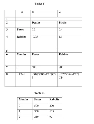
Set up an Excel spread sheets to solve the two differential equations using a first order Euler method. The initial values of the parameters and populations are shown in the figure -1.Copy row 8 down to row 37 to model 30 months. Apply it to the following 3 cases (Table 1) each of which is a different set if initial conditions.
Table: 1
Starting populations
Case Rabbits Foxes
1. 200 500
2. 550 220
3. 500 200
Case 1: Foxes-500; Rabbits -200
Table: 2
Table :3
Months Foxes Rabbits
0 500 200
1 330 135
2 219 92
A B C
1
2 Deaths Births
3 Foxes 0.5 0.4
4 Rabbits -0.75 1.1
5
6 Months Foxes Rabbits
7 0 500 200
8 =A7+1 =$B$3*B7+C7*$C$ 3
ISSN: 2231 – 5373
http://www.ijmttjournal.org
Page 126
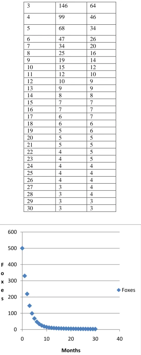
3 146 64
4 99 46
5 68 34
6 47 26
7 34 20
8 25 16
9 19 14
10 15 12
11 12 10
12 10 9
13 9 9
14 8 8
15 7 7
16 7 7
17 6 7
18 6 6
19 5 6
20 5 5
21 5 5
22 4 5
23 4 5
24 4 4
25 4 4
26 4 4
27 3 4
28 3 4
29 3 3
30 3 3
Figure 1: Fox populations over 30 month span starting with 500 foxes
0 100 200 300 400 500 600
0 10 20 30 40
F o x e s
Months
ISSN: 2231 – 5373
http://www.ijmttjournal.org
Page 127
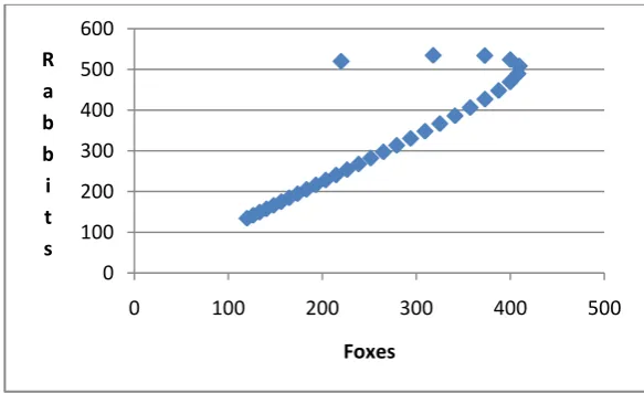
Figure 2:Rabbit populations over 30 months span starting with200 rabbitsFigure 3: Rabbit and Fox population over 30 months span starting with 200 rabbits and 500foxes
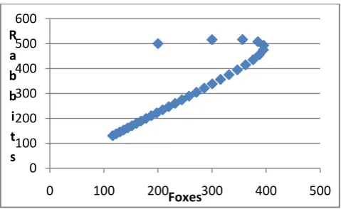
Case : 2 Foxes-220 ; Rabbits-500
Figure 4: Rabbit and Fox population over 30 months span starting with 220 rabbits and 550 foxes
0 50 100 150 200 250
0 10 20 30 40
R a b b i t s
Months
Rabbits
0 50 100 150 200 250
0 200 400 600
R a b b i t s
Foxes
0 100 200 300 400 500 600
0 100 200 300 400 500
R a b b i t s
ISSN: 2231 – 5373
http://www.ijmttjournal.org
Page 128
Case:3 Foxes- 200;Rabbits-500
Figure 5: Rabbit and Fox population over 30 months span starting with 500 rabbits and 200 foxes IV. RESULTS AND DISCUSSION
In case 1 we started with a rabbit population prey of 200 and a predator population foxes of 500.In figure 3 the curve formed in the graph of rabbits verses foxes is called a trajectory of the system. Notice that the curve tends towards the origin ( 0 foxes and 0 rabbits). This means that both species eventually die out. This also shown in the figures 4 and 5 .Change the initial populations from case 2 and case 3 and observe that the trajectories also tend towards the origin.
Over all these various scenarios, using the Euler method, certain overriding trends can be seen. The graph and figures support the notion that the rabbit population and fox population are codependent on one another .The graphs show the number of rabbits present at any moment is related to the number of foxes present at any moment and vice versa. The periodicity of the population depends on the initial values but is regular and consistent in all cases.
V. CONCLUSION
This predator prey model is a rudimentary model of the complex ecology of this model world;it assumes just one prey for the predator and vice versa. It also assumes no outside influences like diseases, changing conditions, populations and so on.
This model is an excellent tool to teach principles involved in ecology and to show some rather counter- initiative results. It also shows a special relationship betweenbiology and mathematics.
REFERENCES
[1] Taylor, R.J. “prediction “, chapman and Hall ,New york;1984.
[2] Erlinge, S,.G, .Goranson, G,Hogsted, G.Jansson, O.Liberg, J.Loman,I.N.Nilson,T.Vonschants and M.Sylven, “ Can vertebrate
Predators regulate their Prey” American Naturalist 23:125-133.1984.
[3] Kidd, N.A.C.,andG.B.Lewis, “ Can vertebrate Predators regulate their Prey” A. reply. American Naturalist 30: 130: 448-453;1987.
[4] Sinclair, A.R.E., P.D.Olsen and T.D. Red head, “Can Predators regulate small mammal populations” , Evidence from house mouse
outbreaks in Australia.Oikos 59: 382-392;1990.
[5] Skogland, T. “What are the effects of Predators on large ungulate populations”, oikos, 61:401-411,1991.
[6] Byers J.A, American Pronghorn; “Social adaptations and the ghosts of Predators past”. University of Chicago. 1997.
[7] Tailor Ravi; Bhathawala P.H; “ Stability of eigen values for Predator- Prey relationships” .IJAET/Vol- I/Issue-II/ April-June, 2011/
140-149.
[8] Jones and Bartlett, “ Mathematical Modeling with excel”, Brain Albright, Student Edition 2010.
0 100 200 300 400 500 600
0 100 200 300 400 500
R a b b i t s