Provably Accurate Double-Sparse Coding
Thanh V. Nguyen [email protected]
Department of Electrical and Computer Engineering Iowa State University
Ames, IA 50011, USA
Raymond K. W. Wong [email protected]
Department of Statistics Texas A&M University
College Station, TX 77843, USA
Chinmay Hegde [email protected]
Department of Electrical and Computer Engineering Iowa State University
Ames, IA 50011, USA
Editor:Animashree Anandkumar
Abstract
Sparse coding is a crucial subroutine in algorithms for various signal processing, deep learn-ing, and other machine learning applications. The central goal is to learn an overcomplete dictionary that can sparsely represent a given input dataset. However, a key challenge is that storage, transmission, and processing of the learned dictionary can be untenably high if the data dimension is high. In this paper, we consider the double-sparsity model intro-duced by Rubinstein et al. (2010b) where the dictionary itself is the product of a fixed, known basis and a data-adaptive sparse component. First, we introduce a simple algo-rithm for double-sparse coding that can be amenable to efficient implementation via neural architectures. Second, we theoretically analyze its performance and demonstrate asymp-totic sample complexity and running time benefits over existing (provable) approaches for sparse coding. To our knowledge, our work introduces the first computationally efficient algorithm for double-sparse coding that enjoys rigorous statistical guarantees. Finally, we corroborate our theory with several numerical experiments on simulated data, suggesting that our method may be useful for problem sizes encountered in practice.
Keywords: Sparse coding, provable algorithms, unsupervised learning
1. Introduction
1.1. Motivation
Representing signals as sparse linear combinations of atoms from a dictionary is a popular approach in many domains. In this paper, we study the problem of dictionary learning
(also known as sparse coding), where the goal is to learn an efficient basis (dictionary) that represents the underlying class of signals well. In the typical sparse coding setup, the dictionary isovercomplete (i.e., the cardinality of the dictionary exceeds the ambient signal dimension) while the representation issparse (i.e., each signal is encoded by a combination of only a few dictionary atoms.)
c
Sparse coding has a rich history in diverse fields such as signal processing, machine learning, and computational neuroscience. Discovering optimal basis representations of data is a central focus of image analysis (Krim et al., 1999; Elad and Aharon, 2006; Rubinstein et al., 2010a), and dictionary learning has proven widely successful in imaging problems such as denoising, deconvolution, inpainting, and compressive sensing (Elad and Aharon, 2006; Candes and Tao, 2005; Rubinstein et al., 2010a). Sparse coding approaches have also been used as a core building block of deep learning systems for prediction (Gregor and LeCun, 2010; Boureau et al., 2010) and associative memory (Mazumdar and Rawat, 2017). Interestingly, the seminal work by Olshausen and Field (1997) has shown intimate connections between sparse coding and neuroscience: the dictionaries learned from image patches of natural scenes bear remarkable resemblance to spatial receptive fields observed in the mammalian primary visual cortex.
From a mathematical standpoint, the sparse coding problem is formulated as follows. Given p data samples Y = [y(1), y(2), . . . , y(p)] ∈ Rn×p, the goal is to find a dictionary D∈Rn×m (m > n) and corresponding sparse code vectors X= [x(1), x(2), . . . , x(p)]∈Rm×p such that the representation DX fits the data samples as well as possible. Typically, one obtains the dictionary and the code vectors as the solution to the following optimization problem:
min
D,XL(D, X) =
1 2
p X
j=1
ky(j)−Dx(j)k22,
s.t.
p X
j=1
S(x(j))≤S
(1)
where S(·) is some sparsity-inducing penalty function on the code vectors, such as the
`1-norm. The objective function L controls the reconstruction error while the constraint
enforces the sparsity of the representation. However, even a cursory attempt at solving the optimization problem (1) reveals the following obstacles:
The constrained optimization problem (1) involves a non-convex (in fact, bilinear) ob-jective function, as well as potentially non-convex constraints depending on the choice of the sparsity-promoting function S (for example, the `0 function.) Hence, obtaining prov-ably correct algorithms for this problem can be challenging. Indeed, the vast majority of practical approaches for sparse coding have been heuristics (Engan et al., 1999; Aharon et al., 2006; Mairal et al., 2009). Recent works in the theoretical machine learning commu-nity have bucked this trend, providing provably accurate algorithms if certain assumptions are satisfied (Spielman et al., 2012; Agarwal et al., 2014; Arora et al., 2014a, 2015; Sun et al., 2015; B lasiok and Nelson, 2016; law Adamczak, 2016; Chatterji and Bartlett, 2017). However, relatively few of these newer methods have been shown to provide good empirical performance in actual sparse coding problems.
one typically resorts to chop the data into smaller blocks (e.g., partitioning image data into patches) to make the problem manageable.
A related line of research has been devoted to learning dictionaries that obey some type ofstructure. Such structural information can be leveraged to incorporate prior knowledge of underlying signals as well as to resolve computational challenges due to the data dimension. For instance, the dictionary is assumed to be separable, or obey a convolutional structure. One such variant is the double-sparse coding problem (Rubinstein et al., 2010b; Sulam et al., 2016) where the dictionary D itself exhibits a sparse structure. To be specific, the dictionary is expressed as:
D= ΦA,
i.e., it is composed of a known “base dictionary” Φ ∈ Rn×n, and a learned “synthesis” matrix A∈Rn×m whose columns are sparse. The base dictionary Φ is typically any fixed
basis chosen according to domain knowledge, while the synthesis matrix A is column-wise sparse and is to be learned from the data. The basis Φ is typically orthonormal (such as the canonical or wavelet basis); however, there are cases where the base dictionary Φ is overcomplete (Rubinstein et al., 2010b; Sulam et al., 2016).
There are several reasons why such the double-sparsity model can be useful. First, the double-sparsity assumption is rather appealing from a conceptual standpoint, since it lets us combine the knowledge of decades of modeling efforts in harmonic analysis with the flexibility of learning new representations tailored to specific data families. Moreover, such a double-sparsity model has computational benefits. If the columns of A are (say)
r-sparse (i.e., each column contains no more than r n non-zeroes) then the overall burden of storing, transmitting, and computing withA is much lower than that for general unstructured dictionaries. Finally, such a model lends itself well to interpretable learned features if the atoms of the base dictionary are semantically meaningful.
All the above reasons have spurred researchers to develop a series of algorithms to learn doubly-sparse codes (Rubinstein et al., 2010b; Sulam et al., 2016). However, despite their empirical promise, no theoretical analysis of their performance have been reported in the literature and to date, we are unaware of a provably accurate, polynomial-time algorithm for the double-sparse coding problem. Our goal in this paper is precisely to fill this gap.
1.2. Our Contributions
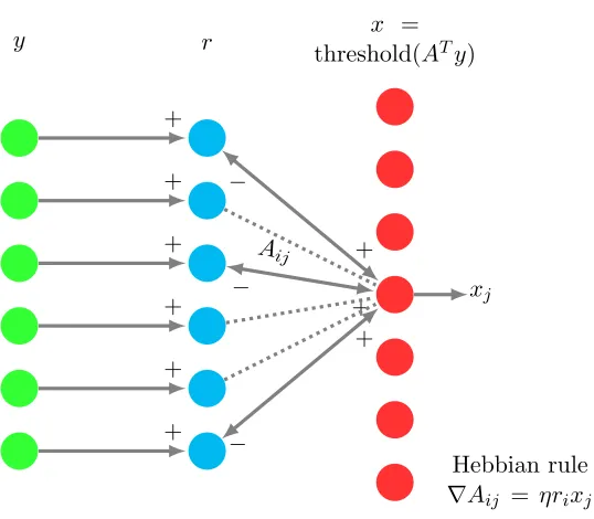
In this paper, we provide a new framework for double-sparse coding. To the best of our knowledge, our approach is the first method that enjoysprovablestatistical and algorithmic guarantees for this problem. In addition, our approach enjoys two benefits: we demonstrate that the method is neurally plausible (i.e., its execution can plausibly be achieved using a neural network architecture) androbust to noise.
Inspired by the aforementioned recent theoretical advances in sparse coding, we assume a learning-theoretic setup where the data samples arise from a ground-truth generative model. Informally, suppose there exists a true (but unknown) synthesis matrix A∗ that is column-wise r-sparse, and theith data sample is generated as:
where the code vectorx∗(i)is independently drawn from a distribution supported on the set of k-sparse vectors. We desire to learn the underlying matrix A∗. Informally, suppose that the synthesis matrixA∗ isincoherent (the columns ofA∗ are sufficiently close to orthogonal) and has bounded spectral norm. Finally, suppose that the number of dictionary elements,
m, is at most a constant multiple of n. All of these assumptions are standard1.
We will demonstrate that the true synthesis matrix A∗ can be recovered (with small error) in a tractable manner as sufficiently many samples are provided. Specifically, we make the following novel contributions:
1. We propose a new algorithm that produces a coarse estimate of the synthesis matrix that is sufficiently close to the ground truth A∗. Our algorithm builds upon spectral initialization-based ideas that have recently gained popularity in non-convex machine learning (Zhang et al., 2016; Wang et al., 2016).
2. Given the above coarse estimate of the synthesis matrix A∗, we propose a descent-style algorithm to refine the above estimate of A∗. This algorithm is simpler than previously studied double-sparse coding algorithms (such as the Trainlets approach of Sulam et al. (2016)), while still giving good statistical performance. Moreover, this algorithm can be realized in a manner amenable to neural implementations.
3. We provide a rigorous analysis of both algorithms. Put together, our analysis produces the first provably polynomial-time algorithm for double-sparse coding. We show that the algorithm provably returns a good estimate of the ground-truth; in particular, in the absence of noise we prove that Ω(mr polylogn) samples are sufficient for a good enough initialization in the first algorithm, as well as guaranteed linear convergence of the descent phase up to a precise error parameter that can be interpreted as the radius of convergence.
Indeed, our analysis shows that employing the double-sparsity model helps in this context, and leads to a strict improvement in sample complexity, as well as running time over previous rigorous methods for (regular) sparse coding such as Arora et al. (2015).
4. We also analyze our approach in a more realistic setting with the presence of additive noise and demonstrate its stability. We prove that Ω(mr polylog n) samples are sufficient to obtain a good enough estimate in the initialization, and also to obtain guaranteed linear convergence during descent to provably recover A∗.
5. We underline the benefit of the double-sparse structure over the regular model by analyzing the algorithms in Arora et al. (2015) under the noisy setting. As a result, we obtain the sample complexity O (mk+σ2εmnk2)polylog n
, which demonstrates a negative effect of noise on this approach.
6. We rigorously develop a hard thresholding intialization that extends the spectral scheme in Arora et al. (2015). Additionally, we provide more results for the case whereA is orthonormal, sparse dictionary to relax the condition onr, which may be of independent interest.
Setting Reference Sample (w/o noise)
Sample
(w/ noise) Time Expt
Regular
MOD (Engan et al., 1999) 7 7 7 3
K-SVD (Aharon et al., 2006) 7 7 7 3
Spielman et al. (2012) O(n2logn) 7
e
Ω(n4) 3
Arora et al. (2014b) Oe(m2/k2) 7 Oe(np2) 7
Gribonval et al. (2015a) O(nm3) O(nm3) 7 7
Arora et al. (2015) Oe(mk) 7 Oe(mn2p) 7
Double Sparse
Double Sparsity (Rubinstein et al., 2010b) 7 7 7 3
Gribonval et al. (2015b) Oe(mr) Oe(mr) 7 7
Trainlets (Sulam et al., 2016) 7 7 7 3
This paper Oe(mr) Oe(mr+σ2εmnr
k ) Oe(mnp) 3
Table 1: Comparison of various sparse coding techniques. Expt: whether numerical experiments have been conducted. 7 in all other columns indicates no provable guarantees. Here,nis the signal dimension, andm is the number of atoms. The sparsity levels forAandxare
randkrespectively, and pis the sample size.
7. While our analysis mainly consists of sufficiency results and involves unknown con-stants hidden in big-O notation, we demonstrate our findings by reporting a suite of numerical experiments on synthetic test datasets.
Overall, our approach results in strict improvement in sample complexity, as well as running time, over previous rigorously analyzed methods for (regular) sparse coding, such as Arora et al. (2015). See Table 1 for a detailed comparison.
1.3. Techniques
At a high level, our method is an adaptation of the seminal approach of Arora et al. (2015). As is common in the statistical learning literature, we assume a “ground-truth” generative model for the observed data samples, and attempt to estimate the parameters of the generative model given a sufficient number of samples. In our case, the parameters correspond to the synthesis matrixA∗, which is column-wiser-sparse. The natural approach is to formulate a loss function in terms of A such as Equation (1), and perform gradient descent with respect to the surface of the loss function to learnA∗.
The key challenge in sparse coding is that the gradient is inherently coupled with the
of the loss, and obtain a descent property directly related to (the population parameter)
A∗.
The second stage of our approach (i.e., our descent-style algorithm) leverages this in-tuition. However, instead of standard gradient descent, we perform approximateprojected
gradient descent, such that the column-wise r-sparsity property is enforced in each new estimate of A∗. Indeed, such an extra projection step is critical in showing a sample com-plexity improvement over the existing approach of Arora et al. (2015).The key novelty is in figuring out how to perform the projection in each gradient iteration. For this purpose, we develop a novel initialization algorithm that identifies the locations of the non-zeroes in A∗
even before commencing the descent phase. This is nontrivially different from initialization schemes used in previous rigorous methods for sparse coding, and the analysis is somewhat more involved.
In Arora et al. (2015), (the principal eigenvector of) a weighted covariance matrix of y
(estimated by the weighted average of outer products yiyTi ) is shown to provide a coarse
estimate of a dictionary atom. We extend this idea and rigoriously show that the diagonal of the weighted covariance matrix serves as a good indicator of the support of a column in A∗. The success relies on the concentration of the diagonal vector with dimension n, instead of the covariance matrix with dimensions n×n. With the support selected, our scheme only utilizes a reduced weighted covariance matrix with dimensions at mostr×r. This initialization scheme enables us to effectively reduce the dimension of the problem, and therefore leads to significant improvement in sample complexity and running time over previous (provable) sparse coding methods when the data representation sparsitykis much smaller than m.
Further, we rigorously analyze the proposed algorithms in the presence of noise with a bounded expected norm. Our analysis shows that our method is stable, and in the case of i.i.d. Gaussian noise with bounded expected`2-norms, is at least a polynomial factor better
than previous polynomial time algorithms for sparse coding.
The empirical performance of our proposed method is demonstrated by a suite of numer-ical experiments on synthetic datasets. In particular, we show that our proposed methods are simple and practical, and improve upon previous provable algorithms for sparse coding.
1.4. Paper Organization
2. Setup and Main Results
2.1. Notation
We define [m],{1, . . . , m} for any integer m > 1. For any vectorx= [x1, x2, . . . , xm]T ∈ Rm, we write supp(x) , {i ∈ [m] : xi 6= 0} as the support set of x. Given any subset S ⊆[m],xScorresponds to the sub-vector ofxindexed by the elements ofS. For any matrix A∈Rn×m, we useA•i and ATj• to represent thei-th column and the j-th row respectively.
For some appropriate setsR andS, letAR• (respectively,A•S) be the submatrix ofAwith
rows (respectively columns) indexed by the elements in R (respectively S). In addition, for the i-th column A•i, we use AR,i to denote the sub-vector indexed by the elements of R. For notational simplicity, we useATR• to indicate (AR•)T, the tranpose ofA after a row
selection. Besides, we use ◦ and sgn(·) to represent the element-wise Hadamard operator and the element-wise sign function respectively. Further, thresholdK(x) is a thresholding
operator that replaces any elements of x with magnitude less thanK by zero.
The `2-norm kxk for a vector x and the spectral norm kAk for a matrix A appear
several times. In some cases, we also utilize the Frobenius norm kAkF and the operator norm kAk1,2 , maxkxk1≤1kAxk. The norm kAk1,2 is essentially the maximal Euclidean
norm of any column ofA.
For clarity, we adopt asymptotic notations extensively. We write f(n) = O(g(n)) (or f(n) = Ω(g(n))) if f(n) is upper bounded (respectively, lower bounded) by g(n) up to some positive constant. Next, f(n) = Θ(g(n)) if and only if f(n) = O(g(n)) and
f(n) = Ω(g(n)). Also Ω ande Oe represent Ω and O up to a multiplicative poly-logarithmic
factor respectively. Finally f(n) = o(g(n)) (or f(n) = ω(g(n))) if limn→∞|f(n)/g(n)|= 0
(limn→∞|f(n)/g(n)|=∞).
Throughout the paper, we use the phrase “with high probability” (abbreviated to w.h.p.) to describe an event with failure probability of order at most n−ω(1). In addition, g(n) =
O∗(f(n)) means g(n)≤Kf(n) for some small enough constantK.
2.2. Generative Model of Data
Suppose that the observed samples are given by
y(i)=Dx∗(i)+ε, i= 1, . . . , p,
i.e., we are givenp samples ofy generated from a fixed (but unknown) dictionary Dwhere the sparse codex∗and the errorεare drawn from a joint distributionDspecified below. In the double-sparse setting, the dictionary is assumed to follow a decomposition D = ΦA∗, where Φ ∈ Rn×n is a known orthonormal basis matrix and A∗ is an unknown, ground
truth synthesis matrix. An alternative (and interesting) setting is an overcomplete Φ with a square A∗, which our analysis below does not cover; we defer this to future work. Our approach relies upon the following assumptions on the synthesis dictionaryA∗:
A1 A∗ is overcomplete (i.e.,m≥n) withm=O(n).
A2 A∗ isµ-incoherent, i.e., for alli6=j,|hA∗•i, A∗•ji| ≤µ/ √
n.
A4 A∗ has bounded spectral norm such thatkA∗k ≤O(pm/n).
All these assumptions are standard. In Assumption A2, the incoherence µ is typically of order O(logn) with high probability for a normal random matrix (Arora et al., 2014b). Assumption A3is a common assumption in sparse signal recovery. The bounded spectral norm assumption is also standard (Arora et al., 2015). In addition to AssumptionsA1-A4, we make the following distributional assumptions on D:
B1 SupportS = supp(x∗) is of size at most kand uniformly drawn without replacement from [m] such thatP[i∈S] = Θ(k/m) andP[i, j∈S] = Θ(k2/m2) for somei, j∈[m]
and i6=j.
B2 The nonzero entriesx∗S are pairwise independent and sub-Gaussian given the support
S with E[x∗i|i∈S] = 0 andE[x∗i2|i∈S] = 1. B3 Fori∈S,|x∗i| ≥C where 0< C≤1.
B4 The additive noiseεhas i.i.d. Gaussian entries with variance σε2 withσε=O(1/ √
n).
For the rest of the paper, we set Φ =In, the identity matrix of sizen. This only simplifies
the arguments but does not change the problem because one can study an equivalent model:
y0=Ax∗+ε0,
where y0 = ΦTy and ε0 = ΦTε, as ΦTΦ = In. Due to the Gaussianity of ε, ε0 also has
independent entries. Although this property is specific to Gaussian noise, all the analysis carried out below can be extended to sub-Gaussian noise with minor (but rather tedious) changes in concentration arguments.
Our goal is to devise an algorithm that produces a provably “good” estimate ofA∗. For this, we need to define a suitable measure of “goodness”. We use the following notion of distance that measures the maximal column-wise difference in`2-norm under some suitable
transformation.
Definition 1 ((δ, κ)-nearness) A is said to be δ-close to A∗ if there is a permutation π: [m]→[m]and a sign flip σ : [m] :{±1} such thatkσ(i)A•π(i)−A∗•ik ≤δ for everyi. In addition, A is said to be (δ, κ)-near to A∗ if kA•π−A∗k ≤κkA∗k also holds.
For notational simplicity, in our theorems we simply replace π and σ in Definition 1 with the identity permutation π(i) = i and the positive sign σ(·) = +1 while keeping in mind that in reality we are referring to one element of the equivalence class of all permutations and sign flip transforms ofA∗.
We will also need some technical tools from Arora et al. (2015) to analyze our gradient descent-style method. Consider any iterative algorithm that looks for a desired solution
z∗ ∈Rn to optimize some functionf(z). Suppose that the algorithm produces a sequence
of estimates z1, . . . , zs via the update rule:
zs+1 =zs−ηgs,
for some vector gs and scalar step size η. The goal is to characterize “good” directions gs
Definition 2 A vector gs at thesth iteration is(α, β, γs)-correlated with a desired solution z∗ if
hgs, zs−z∗i ≥αkzs−z∗k2+βkgsk2−γs.
We know from convex optimization that iffis 2α-strongly convex and 1/2β-smooth, and
gs is chosen as the gradient ∇zf(z), thengs is (α, β,0)-correlated with z∗. In our setting,
the desired solution corresponds to A∗, the ground-truth synthesis matrix. In Arora et al. (2015), it is shown thatgs=Ey[(Asx−y)sgn(x)T], wherex= thresholdC/2((As)Ty) indeed
satisfies Definition 2. This gs is a population quantity and not explicitly available, but
one can estimate such gs using an empirical average. The corresponding estimator bgs is a random variable, so we also need a relatedcorrelated-with-high-probability condition:
Definition 3 A directionbgs at thesthiteration is(α, β, γs)-correlated-w.h.p. with a desired solution z∗ if, w.h.p.,
hgbs, zs−z∗i ≥αkzs−z∗k2+βkbgsk2−γs.
From Definition 2, one can establish a form of descent property in each update step, as shown in Theorem 1.
Theorem 1 Suppose thatgssatisfies the condition described in Definition 2 fors= 1,2, . . . , T. Moreover, 0< η≤2β andγ = maxTs=1γs. Then, the following holds for all s:
kzs+1−z∗k2≤(1−2αη)kzs−z∗k2+ 2ηγs.
In particular, the above update converges geometrically to z∗ with an error γ/α. That is,
kzs+1−z∗k2 ≤(1−2αη)skz0−z∗k2+ 2γ/α.
We can obtain a similar result for Definition 3 except thatkzs+1−z∗k2 is replaced with its
expectation.
Armed with the above tools, we now state some informal versions of our main results:
Theorem 2 (Provably correct initialization, informal) There exists a neurally plau-sible algorithm to produce an initial estimate A0 that has the correct support and is (δ,2) -near to A∗ with high probability. Its running time and sample complexity are Oe(mnp) and
e
O(mr) respectively. This algorithm works when the sparsity level satisfies r=O∗(logn).
step for every learned atom. We obtain the same order restriction onr, but somewhat worse bounds on sample complexity and running time. The details are found in Appendix F.
We hypothesize that a stronger incoherence assumption can lead to provably correct initialization for a much wider range ofr. For purposes of theoretical analysis, we consider the special case of a perfectly incoherent synthesis matrix A∗ such that µ= 0 and m =n. In this case, we can indeed improve the sparsity parameter tor =O∗ min(
√ n log2n,
n k2log2n)
, which is an exponential improvement. This analysis is given in Appendix E.
The next theorem summarizes our result for the descent algorithm:
Theorem 3 (Provably correct descent, informal) There exists a neurally plausible al-gorithm for double-sparse coding that converges to A∗ with geometric rate when the initial estimate A0 has the correct support and (δ,2)-near to A∗. The running time per iteration is O(mkp+mrp) and the sample complexity is Oe(m+σε2mnrk ).
Similar to Arora et al. (2015), our proposed algorithm enjoys neural plausibility. More-over, we can achieve a better running time and sample complexity per iteration than previ-ous methods, particularly in the noisy case. We show in Appendix F that in this regime the sample complexity of Arora et al. (2015) isOe(m+σε2mn
2
k ). For instance, whenσεn −1/2,
the sample complexity bound is significantly worse than Oe(m) in the noiseless case. In
contrast, our proposed method leverages the sparse structure to overcome this problem and obtain improved results.
We are now ready to introduce our methods in detail. As discussed above, our approach consists of two stages: an initialization algorithm that produces a coarse estimate of A∗, and a descent-style algorithm that refines this estimate to accurately recover A∗.
3. Stage 1: Initialization
In this section, we present a neurally plausible algorithm that can produce a coarse initial estimate of the ground truth A∗. We give a neural implementation of the algorithm in Appendix G.
Our algorithm is an adaptation from the algorithm in Arora et al. (2015). The idea is to estimate dictionary atoms in a greedy fashion by iteratively re-weighting the given samples. The samples are re-scaled in a way that the weighted (sample) covariance matrix has the dominant first singular value, and its corresponding eigenvector is close to one particular atom with high probability. However, while this algorithm is conceptually very appealing, it incurs severe computational costs in practice. More precisely, the overall running time is
e
O(mn2p) in expectation, which is unrealistic for large-scale problems.
Algorithm 1 Truncated Pairwise Reweighting
Initialize L=∅
Randomly dividepsamples into two disjoint setsP1 andP2of sizesp1 andp2respectively While |L|< m. Pick uand v from P1 at random
For every l= 1,2, . . . , n; compute
b el=
1
p2 p2
X
i=1
hy(i), uihy(i), vi(yl(i))2
Sort (be1,be2, . . . ,ben) in descending order
If r0 ≤r s.t be(r0)≥O(k/mr) and be(r0+1)/eb(r0)< O
∗(r/log2n)
LetRb be set of the r0 largest entries of be
c
Mu,v= p12 Ppi=12 hy(i), uihy(i), viy (i)
b
R (y (i)
b
R ) T
δ1, δ2← top singular values of Mcu,v z
b
R← top singular vector of Mcu,v If δ1 ≥Ω(k/m) and δ2< O∗(k/mlogn)
If dist(±z, l)>1/lognfor any l∈L
UpdateL=L∪ {z}
Return A0= (L1, . . . , Lm)
Let us provide some intuition of our algorithm. Fix a sample y =A∗x∗ +ε from the available training set, and consider samples
u=A∗α+εu, v=A∗α0+εv.
Now, consider the (very coarse) estimate for the sparse code ofu with respect toA∗:
β=A∗Tu=A∗TA∗α+A∗Tεu.
As long as A∗ is incoherent enough and εu is small, the estimate β behaves just likeα, in
the sense that for each sampley:
hy, ui ≈ hx∗, βi ≈ hx∗, αi.
Moreover, the above inner products are large only if αand x∗ share some elements in their supports; else, they are likely to be small. Likewise, the weight hy, uihy, vi depends on whether or not x∗ shares the support with bothα and α0.
should be sparse as well. Therefore, we can naturally perform an extra “sparsification” step of the output. An extended algorithm and its correctness are provided in Appendix F. However, as we discussed above, the computational complexity of the re-weighting step still remains.
We overcome this obstacle by first identifying the locations of the nonzero entries in each atom. Specifically, define the matrix:
Mu,v =
1
p2 p2
X
i=1
hy(i), uihy(i), viy(i)y(i)T.
Then, the diagonal entries of Mu,v reveals the support of the atom of A∗ shared among u and v: the r-largest entries of Mu,v will correspond to the support we seek. Since the
desired direction remains unchanged in ther-dimensional subspace of its nonzero elements, we can restrict our attention to this subspace, construct a reduced covariance matrixMcu,v,
and proceed as before. This truncation step alleviates the computational burden by a significant amount; the running time is now Oe(mnp), which improves the original by a
factor of n.
The success of the above procedure relies upon whether or not we can isolate pairsuand
v that share one dictionary atom. Fortunately, this can be done via checking the decay of the singular values of the (reduced) covariance matrix. Here too, we show via our analysis that the truncation step plays an important role. Overall, our proposed algorithm not only accelerates the initialization in terms of running time, but also improves the sample complexity over Arora et al. (2015). The performance of Algorithm 1 is described in the following theorem, whose formal proof is deferred to Appendix B.
Theorem 4 Suppose that Assumptions B1-B4 hold and Assumptions A1-A3 satify with µ = O∗
√ n klog3n
and r = O∗(logn). When p1 = Ω(e m) and p2 = Ω(e mr), then with high probability Algorithm 1 returns an initial estimateA0 whose columns share the same support as A∗ and with (δ,2)-nearness toA∗ with δ=O∗(1/logn).
The limit onr arises from the minimum non-zero coefficientτ ofA∗. Since the columns ofA∗ are standardized, τ should degenerate asr grows. In other words, it is getting harder to distinguish the “signal” coefficients from zero asr grows withn. However, this limitation can be relaxed when a better incoherence available, for example the orthonormal case. We study this in Appendix E.
To provide some intuition about the working of the algorithm (and its proof), let us analyze it in the case where we have access to infinite number of samples. This setting, of course, is unrealistic. However, the analysis is much simpler and more transparent since we can focus on expected values rather than empirical averages. Moreover, the analysis reveals several key lemmas, which we will reuse extensively for proving Theorem 4. First, we give some intuition behind the definition of the “scores”,bel.
Lemma 1 Fix samples u and v and suppose that y =A∗x∗+ε is a random sample inde-pendent of u, v. The expected value of the score for the`th component ofy is given by:
el,E[hy, uihy, viyl2] = X
i∈U∩V
qiciβiβi0A ∗2
where qi = P[i ∈ S], qij = P[i, j ∈ S] and ci = E[x4i|i ∈ S]. Moreover, the perturbation terms have absolute value at most O∗(k/mlogn).
From Assumption B1, we know that qi = Θ(k/m), qij = Θ(k2/m2) and ci = Θ(1).
Besides, we will show later that |βi| ≈ |αi| = Ω(1) for i ∈ U, and |βi| = o(1) for i /∈ U.
Consider the first term E0 = Pi∈U∩V qiciβiβi0A∗li2. Clearly, E0 = 0 if U ∩V = ∅ or that l does not belong to support of any atom in U ∩V. On the contrary, as E0 6= 0 and
U ∩V = {i} , then E0 =|qiciβiβ0iAli∗2| ≥ Ω(τ2k/m) = Ω(k/mr) since |qiciβiβi0| ≥Ω(k/m)
and |A∗li| ≥τ.
Therefore, Lemma 1 suggests that if u and v share a unique atom among their sparse representations, and r is not too large, then we can indeed recover the correct support of the shared atom. When this is the case, the expected scores corresponding to the nonzero elements of the shared atom will dominate the remaining of the scores.
Now, given that we can isolate the supportR of the corresponding atom, the remaining questions are how best we can estimate its non-zero coefficients, and whenu andv share a unique elements in their supports. These issues are handled in the following lemmas.
Lemma 2 Suppose that u = A∗α+εu and v = A∗α0+εv are two random samples. Let U and V denote the supports of α and α0 respectively. R is the support of some atom of interest. The truncated re-weighting matrix is formulated as
Mu,v ,E[hy, uihy, viyRyRT] = X
i∈U∩V
qiciβiβi0A ∗ R,iA
∗T
R,i+ perturbation terms
where the perturbation terms have norms at most O∗(k/mlogn).
Using the same argument for boundingE0in Lemma 1, we can see thatM0 ,qiciβiβi0A∗R,iA∗TR,i
has norm at least Ω(k/m) when uand v share a unique elementi(kA∗R,ik= 1). According to this lemma, the spectral norm of M0 dominates those of the other perturbation terms. Thus, given R we can use the first singular vector ofMu,v as an estimate ofA∗•i.
Lemma 3 Under the setup of Theorem 4, suppose u = A∗α+εu and v =A∗α0+εv are two random samples with supports U and V respectively. R = supp(A∗i). If u and v share the unique atom i, the first r largest entries of el is at least Ω(k/mr) and belong to R. Moreover, the top singular vector of Mu,v is δ-close toA∗R,i for O∗(1/logn).
Proof The recovery of A∗•i’s support directly follows Lemma 1. For the latter part, recall from Lemma 2 that
Mu,v =qiciβiβi0A ∗ R,iA
∗T
R,i+ perturbation terms
The perturbation terms have norms bounded by O∗(k/mlogn). On the other hand, the first term is has norm at least Ω(k/m) since kA∗R,ik = 1 for the correct support R and |qiciβiβi0| ≥Ω(k/m). Then using Wedin’s Theorem to Mu,v, we can conclude that the top
Lemma 4 Under the setup of Theorem 4, suppose u = A∗α+εu and v =A∗α0+εv are two random samples with supports U and V respectively. If the top singular value of Mu,v is at least Ω(k/m) and the second largest one is at most O∗(k/mlogn), then uand v share a unique dictionary element with high probability.
Proof The proof follows from that of Lemma 37 in Arora et al. (2015). The main idea is to separate the possible cases of how u and v share support and to use Lemma 2 with the bounded perturbation terms to conclude whenuandvshare exactly one. We note that due to the condition where be(s) ≥Ω(k/mr) andbe(s+1)/be(s) ≤O∗(r/logn), it must be the case that u and v share only one atom or share more than one atoms with the same support. When their supports overlap more than one, then the first singular value cannot dominate
the second one, and hence it must not be the case.
Similar to (Arora et al., 2015), our initialization algorithm requires Oe(m) iterations in
expectation to estimate all the atoms, hence the expected running time isOe(mnp). All the
proofs of Lemma 1 and 2 are deferred to Appendix B.
4. Stage 2: Descent
We now adapt the neural sparse coding approach of Arora et al. (2015) to obtain an improved estimate of A∗. As mentioned earlier, at a high level the algorithm is akin to performing approximate gradient descent. The insight is that within a small enough neighborhood (in the sense ofδ-closeness) of the true A∗, an estimate of the ground-truth code vectors, X∗, can be constructed using a neurally plausible algorithm.
The innovation, in our case, is the double-sparsity model since we know a priori that
A∗ is itself sparse. Under sufficiently many samples, the support of A∗ can be deduced from the initialization stage; therefore we perform an extraprojection step in each iteration of gradient descent. In this sense, our method is non-trivially different from Arora et al. (2015). The full algorithm is presented as Algorithm 2.
As discussed in Section 2, convergence of noisy approximate gradient descent can be achieved as long as bgs is correlated-w.h.p. with the true solution. However, an analogous convergence result for projected gradient descent does not exist in the literature. We fill this gap via a careful analysis. Due to the projection, we only require the correlated-w.h.p. property forpart of bgs (i.e., when it is restricted to some support set) with A∗. The descent property is still achieved via Theorem 5. Due to various perturbation terms, bg
is only a biased estimate of ∇AL(A, X); therefore, we can only refine the estimate of A∗
until the column-wise error is of order O(pk/n). The performance of Algorithm 2 can be characterized via the following theorem.
Theorem 5 Suppose that the initial estimate A0 has the correct column supports and is
(δ,2)-near to A∗ with δ = O∗(1/logn). If Algorithm 2 is provided with p = Ω(e mr) fresh samples at each step and η= Θ(m/k), then
E[kAs•i−A∗•ik2]≤(1−ρ)skA0•i−A∗•ik2+O( p
k/n)
Algorithm 2 Double-Sparse Coding Descent Algorithm
Initialize A0 is (δ,2)-near to A∗. H = (hij)n×m where hij = 1 if i ∈supp(A0•j) and 0
otherwise.
Repeat fors= 0,1, . . . , T
Decode: x(i)= thresholdC/2((As)Ty(i)) fori= 1,2, . . . , p
Update: As+1=PH(As−ηgbs) =As−ηPH(bgs) wheregb
s= 1 p
Pp
i=1(Asx(i)−y(i))sgn(x(i))T and PH(G) =H◦G
We defer the full proof of Theorem 5 to Section D. In this section, we take a step towards understanding the algorithm by analyzingbgs in the infinite sample case, which is equivalent to its expectation gs ,
E[(Asx−y)sgn(x)T]. We establish the (α, β, γs)-correlation of a
truncated version ofg•is withA∗•i to obtain the descent in Theorem 6 for the infinite sample case.
Theorem 6 Suppose that the initial estimate A0 has the correct column supports and is
(δ,2)-near to A∗. If Algorithm 2 is provided with infinite number of samples at each step and η= Θ(m/k), then
kAs•i+1−A∗•ik2 ≤(1−ρ)kAs•i−A∗•ik2+O k2/n2
for some0< ρ <1/2and fors= 1,2, . . . , T. Consequently, it converges toA∗ geometrically until column-wise error is O(k/n).
Note that the better error O(k2/n2) is due to the fact that infinitely many samples are given. The termO(pk/n) in Theorem 5 is a trade-off between the accuracy and the sample complexity of the algorithm. The proof of this theorem composes of two steps with two main results: 1) an explicit form of gs (Lemma 5); 2) (α, β, γs)-correlation of column-wise gs withA∗ (Lemma 6). The proof of those lemmas are deferred to Appendix C. Since the correlation primarily relies on the (δ,2)-nearness of As to A∗ that is provided initially and maintained at each step, then we need to argue that the nearness is preserved after each step.
Lemma 5 Suppose that the initial estimate A0 has the correct column supports and is
(δ,2)-near to A∗. The column-wise update has the form gs
R,i =piqi(λsiAR,is −A∗R,i+ξis±ζ) where R= supp(As•i), λis=hAs•i, A∗•ii and
ξis=AsR,−idiag(qij)(As•−i)TA∗•i/qi.
Moreover, ξi has norm bounded by O(k/n) for δ =O∗(1/logn) and ζ is negligible.
We underline that the correct support ofAs allows us to obtain the closed-form expression ofgRs
i,iin terms ofA
s
•iandA∗•i. Likewise, the gradient form suggests thatgs•iis almost equal
topiqi(As•i−A∗•i) (since λsi ≈1), which directs to the desired solutionA∗•i. With Lemma 5,
we will prove the (α, β, γs)-correlation of the approximate gradient to each column A∗•i and
4.1. (α, β, γs)-Correlation
Lemma 6 Suppose that As to be (δ,2)-near to A∗ and R = supp(A∗•i), then 2gR,is is
(α,1/2α, 2/α)-correlated with A∗R,i; that is
h2gR,is , AsR,i−A∗R,ii ≥αkAsR,i−A∗R,ik2+ 1/(2α)kgs
R,ik2−2/α. where δ =O∗(1/logn) and =O mnk2 . Futhermore, the descent is achieved by
kAs•i+1−A∗•ik2 ≤(1−2αη)skA0•i−A∗•ik2+η2/α.
ProofThroughout the proof, we omit the superscriptsfor simplicity and denote 2α=piqi.
First, we rewritegs
•i as a combination of the true directionAs•i−A∗•i and a term with small
norm:
gR,i = 2α(AR,i−A∗R,i) +v, (2)
where v = 2α[(λi −1)A•i +i] with norm bounded. In fact, since A•i is δ-close to A∗•i,
and both have unit norm, then k2α(λi −1)A•ik = αkA•i −A∗•ik2 ≤ αkA•i −A∗•ik and kξik ≤O(k/n) from the inequality (9). Therefore,
kvk=k2α(λi−1)AR,i+ 2αξik ≤αkAR,i−A∗R,ik+
where=O(k2/mn). Now, we make use of (2) to show the first part of Lemma 6: h2gR,i, AR,i−A∗R,ii= 4αkAR,i−A∗R,ik
2
+h2v, AR,i−A∗R,ii. (3)
We want to lower bound the inner product term with respect tokgRi,ik
2andkA
R,i−A∗R,ik 2.
Effectively, from (2)
4αhv, A•i−A∗•ii=kgR,ik2−4α2kAR,i−A∗R,ik 2− k
vk2
≥ kgR,ik2−6α2kAR,i−A∗R,ik2−22, (4)
where the last step is due to Cauchy-Schwarz inequality: kvk2≤2(α2kAR,i−A∗R,ik2+2).
Substitute 2hv, A•i−A∗•ii in (3) for the right hand side of (4), we get the first result:
h2gR,i, AR,i−A∗R,ii ≥αkAR,i−A∗R,ik2+
1 2αkgR,ik
2−2 α.
The second part is directly followed from Theorem 1. Moreover, we have pi = Θ(k/m)
and qi = Θ(1), then α = Θ(k/m), β = Θ(m/k) and γs = O(k3/mn2). Then gsR,i is
(Ω(k/m),Ω(m/k), O(k3/mn2))-correlated with the true solution A∗R,i.
0 2,000 4,000 0
0.2 0.4 0.6 0.8 1 Sample size Reco v ery rate
0 2,000 4,000 0 2 4 6 8 Sample size Reconstruction error Ours Arora Arora+HT Trainlets
0 2,000 4,000 0 1 2 3 4 Sample size Running time (s)
0 2,000 4,000 0
0.2 0.4 0.6 0.8 1 Sample size Reco v ery rate
0 2,000 4,000 0 2 4 6 8 Sample size Reconstruction error Ours Arora Arora+HT Trainlets
0 2,000 4,000 0 2 4 6 Sample size Running time (s)
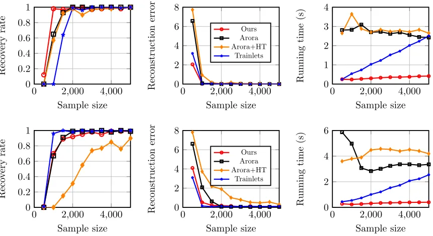
Figure 1: (top) The performance of four methods on three metrics (recovery rate, reconstruction error and running time (in seconds)) in sample size in the noiseless case. (bottom) The same metrics are measured for the noisy case.
4.2. Nearness
Lemma 7 Suppose that As is(δ,2)-near toA∗, then kAs+1−A∗k ≤2kA∗k
Proof [Proof] From Lemma 5 we haveg•is =piqi(λiAs•i−A∗•i) +A•−idiag(qij)AT•−iA∗•i±ζ.
Denote ¯R = [n]\R, then it is obvious thatgs ¯
R,i =AR,−i¯ diag(qij)A T
•−iA∗•i±ζ is bounded by O(k2/m2). Then we follows the proof of Lemma 24 in (Arora et al., 2015) for the nearness
with full gs=gsR,i+gsR,i¯ to finish the proof for this lemma.
In sum, we have shown the descent property of Algorithm 2 in the infinite sample case. The study of the concentration ofgbs around its mean to the sample complexity is provided
in Section D. In the next section, we corroborate our theory by some numerical results on synthetic data.
5. Empirical Study
0 2,000 4,000 0
0.2 0.4 0.6 0.8 1
Sample size
Reco
v
e
ry
rate
0 2,000 4,000 0
0.2 0.4 0.6 0.8 1
Sample size
Reconstruction
error
k=5 k=6 k=7 k=8 k=9
Figure 2: The performance of our method in the noiseless case as the sparsitykvaries.
0 2,000 4,000 0.6
0.8 1
Sample size
Reco
v
ery
rate
0 2,000 4,000 0
0.2 0.4
Sample size
Reconstruction
error
C=0.4 C=0.6 C=0.8 C=1.0 C=1.2
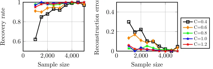
Figure 3: The performance of our method in the noiseless case as the thresholding parameterC varies.
We generate a synthetic training dataset according to the model described in Section 2. The base dictionary Φ is the identity matrix of size n = 64, and the square synthesis matrix A∗ has a special block structure with 32 blocks. Each block is of size 2×2 and of form [1 1; 1 −1] (i.e., the column sparsity of A∗ is r = 2). The support of x∗ is drawn uniformly over all 6-dimensional subsets of [m], and the nonzero coefficients are randomly set to±1 with equal probability. In our simulations with noise, we add Gaussian noiseεwith entrywise varianceσ2ε = 0.01 to each of those above samples. For all the approaches except Trainlets, we use T = 2000 iterations for the initialization procedure, and set the number of steps in the descent stage to 25. Since Trainlets does not have a specified initialization procedure, we initialize it with a random Gaussian matrix upon which column-wise sparse thresholding is then performed. The learning step of Trainlets2is executed for 50 iterations, which tolerates its initialization deficiency. For each Monte Carlo trial, we uniformly draw
p samples, feed these samples to the four different algorithms, and observe their ability to reconstruct A∗. Matlab implementation of our algorithms is available online3.
5.1. Comparison with Other Approaches
We evaluate these approaches on three metrics as a function of the number of available samples: (i) fraction of trials in which each algorithm successfully recovers the ground truth
A∗; (ii) reconstruction error; and (iii) running time (in seconds). The synthesis matrix is said to be “successfully recovered” if the Frobenius norm of the difference between the estimateAband the ground truthA∗ is smaller than a threshold which is set to 10−4 in the
noiseless case, and to 0.5 in the other. All three metrics are averaged over 100 Monte Carlo simulations. As discussed above, the Frobenius norm is only meaningful under a suitable permutation and sign flip transformation linkingAbandA∗. We estimate this transformation
using a simple maximum weight matching algorithm. Specifically, we construct a weighted bipartite graph with nodes representing columns ofA∗ andAband adjacency matrix defined
as G= |A∗TAb|, where |·|is taken element-wise. We compute the optimal matching using
the Hungarian algorithm, and then estimate the sign flips by looking at the sign of the inner products between the matched columns.
The results of our experiments are shown in Figure 1 with the top and bottom rows respectively for the noiseless and noisy cases. The two leftmost figures suggest that all algorithms exhibit a “phase transition” in sample complexity that occurs in the range of 500-2000 samples. In the noiseless case, our method achieves the phase transition with the fewest number of samples. In the noisy case, our method nearly matches the best sample complexity performance (next to Trainlets, which is a heuristic and computationally expensive). Our method achieves the best performance in terms of (wall-clock) running time in all cases.
5.2. Robustness to Data Assumptions
In this last experiement, we show that our approach is robust to the data assumptions. We numerically study how the initialization and descent algorithms behave when the sparsity
kand the thresholding parameterC slightly vary around the groundtruth values. Since our focus is on the recovery property of our approach, we assume that the dictionary size m
and sparsity r are known a priori and do not experiement on them.
The results are shown in Figures 2 and 3. When the sparsity and the minimum coefficient are around the true setting,kmodel= 6 andCmodel= 1.0, our algorithm is still able recover
the dictionary perfectly. When these parameters are set more extreme, the phase transition is not obvious but is gradually achieved with more and more samples.
6. Conclusion
benefits of our approach: neural plausibility, robustness to noise and practical usefulness via the numerical experiments.
Nevertheless, several fundamental questions regarding our approach remain. First, our initialization method (in the overcomplete case) achieves its theoretical guarantees under fairly stringent limitations on the sparsity levelr. This arises due to our reweighted spectral initialization strategy, and it is an open question whether a better initialization strategy exists (or whether these types of initialization are required at all). Second, our analysis holds for complete (fixed) bases Φ, and it remains open to study the setting where Φ is over-complete. Finally, understanding the reasons behind the very promising practical performance of methods based on heuristics, such as Trainlets, on real-world data remains a very challenging open problem.
Acknowledgments
Appendix Organization We organize the appendix as follows: we prove the two key lemmas for Theorem 4 of the initialization algorithm 1 in Appendix B. In Appendix C, we prove the result stated in Theorem 5 for the infinite-sample case. The sample complexity results for both stages are proved in Appendix D.
Additionally, we prove some extended results from Arora et al. (2015) and for some special cases in Appendices E and F. The final section details the neural implementation of our approach.
Appendix A. Useful Result
We start our proof with the following claim, which we will use throughout.
Claim 1 (Maximal row `1-norm) Given that kA∗kF2 =m and kA∗k=O( p
m/n), then kA∗Tk1,2= Θ(pm/n).
Proof Recall the definition of the operator norm:
kA∗Tk1,2 = sup
x6=0
kATxk kxk1 ≤supx6=0
kATxk kxk =kA
∗Tk=O(p m/n).
Since kA∗k2F = m, kA∗Tk1,2 ≥ kA∗kF/√n=pm/n. Combining with the above, we have kA∗Tk1,2= Θ(
p
m/n).
Along with Assumptions A1 and A3, the above claim implies the number of nonzero entries in each row is O(r). This Claim is an important ingredient in our analysis of our initialization algorithm shown in Section 3.
Appendix B. Analysis of Initialization Algorithm
B.1. Proof of Lemma 1
Recall some important notations: y=A∗x∗+εand two samples
u=A∗α+εu, v=A∗α0+εv.
Also, recall the very coarse estimate for the sparse code ofu with respect toA∗:
β=A∗Tu=A∗TA∗α+A∗Tεu.
We split the proof of Lemma 1 into three steps: 1) we first establish useful properties of β
with respect toα; 2) we then explicitly deriveelin terms of the generative model parameters
andβ; and 3) we finally bound the error terms inEbased on the first result and appropriate assumptions.
Claim 2 In the generative model,kx∗k ≤Oe(
√
k)andkεk ≤Oe(σε
√
n)with high probability.
Proof The claim directly follows from the fact that x∗ is a k-sparse random vector whose nonzero entries are independent sub-Gaussian with variance 1. Meanwhile, ε has n
inde-pendent Gaussian entries of varianceσ2ε.
Claim 3 Suppose thatu=A∗α+εu is a random sample andU = supp(α). Letβ =A∗Tu, then, w.h.p., we have (a)|βi−αi| ≤ µk√lognn+σεlognfor eachiand (b)kβk ≤Oe(
√
k+σε √
n).
Proof The proof mostly follows from Claim 36 of Arora et al. (2015), with an additional consideration of the errorεu. WriteW =U\{i}and observe that
|βi−αi|=|A∗T•i A∗•WαW +A•i∗Tεu| ≤ |hA∗T•WA∗•i, αWi|+|hA∗•i, εui|
SinceA∗ isµ-incoherence, thenkA∗T•i A•W∗ k ≤µpk/n. Moreover,αW hask−1 independent
sub-Gaussian entries of variance 1, therefore|hA∗T•WA∗•i, αWi| ≤ µk√lognnwith high probability.
Also recall that εu has independent Gaussian entries of variance σ2ε, then A∗T•i εu is
Gaus-sian with the same variance (kA∗•ik = 1). Hence |A∗T•i ε| ≤ σεlogn with high probability.
Consequently, |βi−αi| ≤ µk√lognn +σεlogn, which is the first part of the claim.
Next, in order to bound kβk, we expressβ as
kβk=kA∗TA•U∗ αU+A∗Tεuk ≤ kA∗kkA∗•UkkαUk+kA∗kkεuk
Using Claim 2 to getkαUk ≤Oe(
√
k) andkεuk ≤Oe(σε
√
n) w.h.p., and further noticing that kA∗•Uk ≤ kA∗k ≤O(1) , we complete the proof for the second part. Claim 3 suggests that the difference betweenβiandαiis bounded above byO∗(1/log2n)
w.h.p. if µ = O∗(
√ n
klog3n). Therefore, w.h.p., C−o(1) ≤ |βi| ≤ |αi|+o(1) ≤O(logm) for i ∈ U and |βi| ≤ O∗(1/log2n) otherwise. On the other hand, under Assumption B4, kβk ≤Oe(
√
k) w.h.p. We will use these results multiple times in the next few proofs.
Proof [Proof of Lemma 1] We decompose dl into small parts so that the stochastic model D is made use.
el=E[hy, uihy, viyl2] =E[hA ∗
x∗+ε, uihA∗x∗+ε, vi(hA∗l·, x∗i+εl)2]
=Ehx∗, βihx∗, β0i+x∗T(βvT +β0uT)ε+uTεεTv hA∗l•, x∗i 2
+ 2hA∗l•, x∗iεl+ε2l
=E1+E2+· · ·+E9
where the terms are
E1=E[hx∗, βihx∗, β0ihA∗l•, x∗i2] E2= 2E[hx∗, βihx∗, β0ihA∗l•, x∗iεl]
E3=E[hx∗, βihx∗, β0iε2l]
E4=EhA∗l·, x∗i2x∗T(βvT +β0uT)ε
E5=EhA∗l·, x∗ix∗T(βvT +β0uT)εεl
E6=E(βvT +β0uT)εε2l
E7=E[uTεεTvhA∗l•, x∗i2] E8= 2E[uTεεTvhA∗l•, x∗iεl]
E9=E[uTεεTvε2l]
Because x∗ and εare independent and zero-mean, E2 andE4 are clearly zero. Moreover, E6 = (βvT +β0uT)E[εε2l] = 0
due to the fact that E[εjε2l] = 0, for j6=l, and E[ε3l] = 0. Also, E8 =A∗Tl• E[x∗]E
uTεεTvεl
= 0.
We bound the remaining terms separately in the following claims.
Claim 4 In the decomposition (5), E1 is of the form
E1= X
i∈U∩V
qiciβiβi0A∗li2+ X
i /∈U∩V
qiciβiβi0A∗li2+ X
j6=i
qij(βiβi0A∗lj2+ 2βiβ0jA∗liA∗lj)
where all those terms except P
i∈U∩V qiciβiβi0A ∗2
li have magnitude at most O
∗(k/mlog2n) w.h.p.
Proof Using the generative model in AssumptionsB1-B4, we have
E1 =E[hx∗, βihx∗, β0ihA∗l•, x∗i2]
=ES
Ex∗|S[ X
i∈S βix∗i
X
i∈S
βi0x∗i X i∈S
A∗lix∗i2]
= X
i∈[m]
qiciβiβi0A ∗2 li +
X
i,j∈[m],j6=i
qij(βiβi0A ∗2
lj + 2βiβj0A ∗ liA ∗ lj) = X i∈U∩V
qiciβiβi0A∗li2+ X
i /∈U∩V
qiciβiβi0A∗li2+ X
j6=i
qij(βiβi0A∗lj2+ 2βiβj0A∗liA∗lj),
where we have used theqi =P[i∈S],qij =P[i, j∈S] andci=E[x4i|i∈S] and Assumptions B1-B4. We now prove that the last three terms are upper bounded byO∗(k/mlogn). The key observation is that all these terms typically involve a quadratic form of the l-th row
A∗l• whose norm is bounded by O(1) (by Claim 1 and Assumption A4). Moreover, |βiβi0|
is relatively small for i /∈U ∩V while qij = Θ(k2/m2). For the second term, we apply the
Claim 3 for i∈[m]\(U ∩V) to bound |βiβi0|. Assume αi = 0 and α0i 6= 0, then with high
probability
|βiβi0| ≤ |(βi−αi)(βi0−α0i)|+|βiαi0| ≤O∗(1/logn)
Using the bound qici = Θ(k/m), we have w.h.p.,
X
i /∈U∩V
qiciβiβi0A ∗2 li
≤maxi |qiciβiβ 0 i|
X
i /∈U∩V
A∗li2 ≤max
i |qiciβiβ 0 i|kA
∗k2 1,2 ≤O
∗(k/mlogn).
For the third term, we make use of the bounds onkβkandkβ0kfrom the previous claim wherekβkkβ0k ≤Oe(k) w.h.p., and onqij = Θ(k2/m2). More precisely, w.h.p.,
X
j6=i
qijβiβi0A ∗2 lj = X i βiβ0i
X
j6=i qijA∗lj2
≤
X
i |βiβ0i|
X
j6=i qijA∗lj2
≤(max
i6=j qij) X
i |βiβi0|
X
j
A∗lj2≤(max
i6=j qij)kβkkβ
0kkA∗k2
where the second last inequality follows from the Cauchy-Schwarz inequality. For the last term, we write it in a matrix form asP
j6=iqijβiβ 0 jA∗liA
∗ lj =A
∗T
l• QβA∗l•where (Qβ)ij =qijβiβj0
fori6=j and (Qβ)ij = 0 for i=j. Then
|A∗Tl• QβA∗l•| ≤ kQβkkA∗l•k2≤ kQβkFkA ∗k2
1,2,
where kQβk2F = P
i6=jqij2βi2(βj0)2 ≤ (maxi6=jqij2) P
iβ2i P
j(βj0)2 ≤ (maxi6=jq2ij)kβk 2kβ0k2.
Ultimately,
X
j6=i
qijβiβj0A∗liA∗lj
≤(maxi6
=j qij)kβkkβ
0kkA∗k2
1,2≤Oe(k3/m2).
Under Assumption k= O∗(
√ n
logn), then Oe(k3/m2) ≤ O∗(k/mlog2n). As a result, the two
terms above are bounded by the same amount O∗(k/mlogn) w.h.p., so we complete the
proof of the claim.
Claim 5 In the decomposition (5), |E3|, |E5|, |E7|and |E9|are at most O∗(k/mlog2n). Proof Recall that E[x2i|S] = 1 and qi =P[i∈S] = Θ(k/m) for S = supp(x
∗), then
E3 =E[hx∗, βihx∗, β0iε2l] =σε2ES
Ex∗|S[ X
i,j∈S βiβj0x
∗ ix
∗ j]
=σε2ES[ X
i∈S
βiβi0] = X
i
σ2εqiβiβi0
DenoteQ= diag(q1, q2, . . . , qm), then|E3|=|σ2εhQβ, β0i| ≤σε2kQkkβkkβ0k ≤Oe(σε2k2/m) = e
O(k3/mn) where we have used kβk ≤Oe(
√
k) w.h.p. and σε ≤O(1/ √
n). For convenience, we handle the seventh term beforeE5:
E7 =E[uTεεTvhA∗l•, x∗i2] =E[hA∗l•, x∗i2]uTE[εεT]v= X
i
σε2hu, viqiA2li =σ2εhu, viATl•QAl•
To bound this term, we use Claim 9 in Appendix D to have kuk= kA∗α+εuk ≤ Oe(
√
k) w.h.p. and hu, vi ≤ Oe(
√
k) w.h.p. Consequently, |E7| ≤ σε2kQkkAl•k2|hu, vi| ≤ Oe(k2/mn)
because kAl•k2 ≤ O(m/n) and σε ≤ O(1/ √
n). Now, the firth term E5 is expressed as
follows
E5=EhA∗l·, x∗ix∗T(βvT +β0uT)εεl
=A∗Tl• Ex∗x∗T(βvT +β0uT)E[εεl]
=σ2εA∗Tl• Q(vlβ+ulβ0)
Observe that |E5| ≤σε2kA∗Tl• kkQ(vlβ+ulβ0)k ≤σε2kA∗Tl• kkQkkvlβ+ulβ0k and that kvlβ+ ulβ0k ≤ 2kukkβk ≤ Oe(k) w.h.p. using the result kuk ≤ Oe(k) and kβk ≤Oe(k) from Claim
3, thenE5 bounded by Oe(k2/mn).
The last term
E9 =E[uTεεTvε2l] =uTE
because the independent entries of ε and E[ε4l] = 9σε4. Therefore, |E9| ≤ 9σε4kukkvk ≤ e
O(k2/n2). Since m =O(n) and k ≤O∗( √n
logn), we obtain the same bound O
∗(k/mlog2n)
for|E3|,|E5|,|E7|and |E9|, and conclude the proof of the claim. Combining the bounds from Claim 4, 5 for every single term in (5), we finish the proof
for Lemma 1.
B.2. Proof of Lemma 2
We prove this lemma by using the same strategy used to prove Lemma 1.
Mu,v ,E[hy, uihy, viyRyRT]
=E[hA∗x∗+ε, uihA∗x∗+ε, vi(A∗R•x∗+εR)(A∗R•x∗+εR)T]
=Ehx∗, βihx∗, β0i+x∗T(βvT +β0uT)ε+uTεεTv A∗R•x∗x∗TA∗TR•+A∗R•x∗εTR+εRx∗TA∗TR•+εRεTR
=M1+· · ·+M8,
in which only nontrivial terms are kept in place, including
M1 =E[hx∗, βihx∗, β0iA∗R•x∗x∗TA∗TR•]
M2 =E[hx∗, βihx∗, β0iεRεTR]
M3 =E[x∗T(βvT +β0uT)εA∗R•x∗εTR]
M4 =E[x∗T(βvT +β0uT)εεRx∗TA∗TR•]
M5 =E[uTεεTvA∗R•x∗x∗TA∗TR•]
M6 =E[uTεεTvA∗R•x∗εTR]
M7 =E[uTεεTvεTRx∗TA∗TR•]
M8 =E[uTεεTvεRεTR]
(6)
By swapping inner product terms and taking advantage of the independence, we can show thatM6 =E[A∗R•x∗uTεεTvεTR] = 0 and M7=E[uTεεTvεTRx
∗TA∗T
R•] = 0. The remaining are
bounded in the next claims.
Claim 6 In the decomposition (6),
M1= X
i∈U∩V
qiciβiβi0A ∗ R,iA
∗T R,i+E
0 1+E
0 2+E
0 3 whereE10 =P
i /∈U∩V qiciβiβi0A∗R,iA∗TR,i,E20 = P
i6=jqijβiβi0A∗R,jA∗TR,j andE30 = P
i6=jqij(βiA∗R,iβj0A∗TR,j+ βi0A∗R,iβjA∗TR,j) have norms bounded by O
∗(k/mlogn).
Proof The expression ofM1 is obtained in the same way as E1 is derived in the proof of
Lemma 1. To prove the claim, we bound all the terms with respect to the spectral norm of
A∗R• and make use of Assumption A4to find the exact upper bound.
For the first termE01, rewriteE10 =A∗R,SD1A∗TR,S whereS = [m]\(U∩V) andD1 is a
di-agonal matrix whose entries areqiciβiβi0. Clearly,kD1k ≤maxi∈S|qiciβiβi0| ≤O∗(k/mlogn)
as shown in Claim 4, then
kE10k ≤max
i∈S|qiciβiβ 0
i|kA∗R,Sk 2 ≤
max
i∈S|qiciβiβ 0
where kA∗R,Sk ≤ kA∗R•k ≤ O(1). The second term E20 is a sum of positive semidefinite matrices, and kβk ≤O(klogn), then
E02=X
i6=j
qijβiβ0iA∗R,jA∗TR,j maxi6 =j qij
X
i βiβi0
X
j
A∗R,jA∗TR,j
(max
i6=j qij)kβkkβ 0kA∗
R•A∗TR•
which implies that kE20k ≤ (maxi6=jqij)kβkkβ0kkA∗R•k2 ≤Oe(k3/m2). Observe thatE30 has
the same form as the last term in Claim 4, which isE30 =A∗TR•QβA∗R•. Then kE30k ≤ kQβkkA∗R•k2 ≤(max
i6=j qij)kβkkβ 0kk
A∗R•k2 ≤Oe(k3/m2)
By Claim 3, we have kβk and kβ0k are bounded by O(√klogn), and note that k ≤
O∗(√n/logn), then we complete the proof for Lemma 6.
Claim 7 In the decomposition (6), M2, M3, M4, M5 and M8 have norms bounded by O∗(k/mlogn).
Proof Recall the definition of Q in Claim 5 and use the fact that E[x∗x∗T] = Q, we can
get M2 = E[hx∗, βihx∗, β0iεRεTR] = P
iσε2qiβiβi0Ir. Then, kM2k ≤ σ2εmaxiqikβkkβ0k ≤ O(σ2εk2log2n/m).
The next three terms all involve A∗R• whose norm is bounded according to Assumption
A4. Specifically,
M3 =E[x∗T(βvT +β0uT)εA∗R•x∗εTR] =E[A ∗
R•x∗x∗T(βvT +β0uT)εεTR]
=A∗R•E[x∗x∗T](βvT +β0uT)E[εεTR]
=A∗R•Q(βvT +β0uT)E[εεTR],
and
M4=E[x∗T(βvT +β0uT)εεRx∗TA∗TR•] =E[εRεT(vβT +uβ0T)x∗x∗TA∗TR•]
=E[εRεT](vβT +uβ0T)E[x∗x∗T]A∗TR•
=E[εRεT](vβT +uβ0T)QA∗TR•,
and the fifth termM5=E[uTεεTvA∗R•x∗x∗TA∗TR•] =σ2εuTvA∗R•E[x∗x∗T]A∗TR• =σ2εuTvA∗R•QA∗TR•.
We already havekE[εεTR]k=σ2ε,kQk ≤O(k/m) and|uTv| ≤Oe(k) (proof of Claim 9), then
the remaining work is to boundkβvT+β0uTk, then the bound ofvβT+uβ0T directly follows. We have kβvTk=kA∗uvTk ≤ kA∗kkukkvk ≤Oe(k). Therefore, all three terms M3,M4 and M5 are bounded in norm by Oe(σ2εk2/m)≤Oe(k3/mn).
The remaining term is
M8 =E[uTεεTvεRεTR] =E[ X
i,j
uivjεiεj
εRεTR]
=E[ X
i∈R
uiviε2iεRεTR
] +E[ X
i6=j
uivjεiεj
εRεTR]
whereuR=A∗R•α+ (εu)R and vR =AR•∗ α0+ (εv)R. We can see that kuRk ≤ kA∗R•kkαk+ k(εu)Rk ≤ Oe(
√
k). Therefore, kM8k ≤ Oe(σε4k) = Oe(k3/n2). Since m = O(n) and k ≤ O∗(
√ n
logn), then we can bound all the above terms byO
∗(k/mlogn) and finish the proof of
Claim 7.
Combine the results of Claim 6 and 7, we complete the proof of Lemma 2.
Appendix C. Analysis of Main Algorithm
C.1. Simple Encoding
We can see that (Asx−y)sgn(x)T is random overyandxthat is obtained from the encoding
step. We follow (Arora et al., 2015) to derive the closed form of gs =E[(Asx−y)sgn(x)T]
by proving that the encoding recovers the sign ofx∗ with high probability as long as As is close enough to A∗.
Lemma 8 Assume that As is δ-close to A∗ for δ = O(r/nlogn) and µ ≤ √
n
2k, and k ≥
Ω(logm) then with high probability over random samplesy=A∗x∗+ε
sgn(thresholdC/2 (As)Ty
= sgn(x∗) (7)
Proof [Proof of Lemma 8] We follow the same proof strategy from (Arora et al., 2015) (Lemmas 16 and 17) to prove a more general version in which the noise ε is taken into account. Write S = supp(x∗) and skip the superscript s on As for the readability. What
we need is to show S = {i ∈ [m] : hA•i, yi ≥ C/2} and then sgn(hAs•i, yi) = sgn(x∗i) for
each i∈S with high probability. Following the same argument of (Arora et al., 2015), we prove in below a stronger statement that, even conditioned on the support S, S = {i ∈ [m] :|hA•i, yi| ≥C/2} with high probability.
Rewrite
hA•i, yi=hA•i, A∗x∗+εi=hA•i, A∗•iix∗i + X
j6=i
hA•i, A∗•jix∗j +hA•i, εi,
and observe that, due to the closeness ofA•i and A∗•i, the first term is either close tox∗i or
equal to 0 depending on whether or not i ∈ S. Meanwhile, the rest are small due to the incoherence and the concentration in the weighted average of noise. We will show that both
Zi =PS\{i}hA•i, A∗•jix∗j andhA•i, εi are bounded by C/8 with high probability.
The cross-termZi =PS\{i}hA•i, A∗•jix∗j is a sum of zero-mean independent sub-Gaussian
random variables, which is another sub-Gaussian random variable with variance σ2Z
i =
P
S\{i}hA•i, A∗•ji2. Note that
hA•i, A∗•ji2 ≤2 hA∗•i, A•j∗ i2+hA•i−A∗•i, A∗•ji2
≤2µ2/n+ 2hA•i−A∗•i, A∗•ji2,
where we use Cauchy-Schwarz inequality and theµ-incoherence of A∗. Therefore,
σZ2i ≤2µ2k/n+ 2kA∗T•S(A•i−A∗•i)k2F ≤2µ
2k/n+ 2kA∗
•Sk2kA•i−A∗•ik2 ≤O(1/logn),
under µ ≤ √
n
2k, to conclude 2µ2k/n ≤ O(1/logn) we need 1/k = O(1/logn), i.e. k =
remains is to bound the noise term hA•i, εi. In fact, hA•i, εi is sum ofn Gaussian random
variables, which is a sub-Gaussian with varianceσ2ε. It is easy to see that|hA•i, εi| ≤σεlogn
with high probability. Notice thatσε =O(1/ √
n).
Finally, we combine these bounds to have |Zi+hA•i, εi| ≤ C/4. Therefore, for i ∈S,
then|hA•i, yi| ≥C/2 and negligible otherwise. Using union bound for everyi= 1,2, . . . , m,
we finish the proof of the Lemma.
Lemma 8 enables us to derive the expected update direction gs=E[(Asx−y)sgn(x)T]
explicitly.
C.2. Approximate Gradient in Expectation
Proof [Proof of Lemma 5] Having the result from Lemma 8, we are now able to study the expected update direction gs =E[(Asx−y)sgn(x)T]. Recall that As is the update at
the s-th iteration and x ,thresholdC/2((As)Ty). Based on the generative model, denote
pi = E[x∗isgn(x∗i)|i ∈ S], qi = P[i ∈ S] and qij =P[i, j ∈ S]. Throughout this section, we
will use ζ to denote any vector whose norm is negligible although they can be different across their appearances. A−i denotes the sub-matrix ofA whosei-th column is removed.
To avoid overwhelming appearance of the superscript s, we skip it from As for neatness.
DenoteFx∗ is the event under which the support ofx is the same as that of x∗, and ¯Fx∗ is
its complement. In other words,1Fx∗ =1[sgn(x) = sgn(x
∗)] and1
Fx∗+1F¯x∗ = 1.
g•is =E[(Ax−y)sgn(xi)] =E[(Ax−y)sgn(xi)1Fx∗]±ζ
Using the fact that y =A∗x∗+εand that underFx∗ we have Ax=A•SxS =A•SAT •Sy= A•SAT•SA∗x∗+A•SAT•Sε. Using the independence ofε and x∗ to get rid of the noise term,
we get
gs•i =E[(A•SAT•S−In)A∗x∗1Fx∗] +E[(A•SAT•S−In)εsgn(xi)1Fx∗]±ζ
=E[(A•SAT•S−In)A∗x∗sgn(xi)1Fx∗]±ζ (Independence of εandx’s)
=E[(A•SAT•S−In)A∗x∗sgn(x∗i)(1−1F¯x∗)]±ζ (UnderFx∗ event)
=E[(A•SAT•S−In)A∗x∗sgn(x∗i)]±ζ
Recall from the generative model assumptions thatS= supp(x∗) is random and the entries of x∗ are pairwise independent given the support, so
gs•i=ESEx∗|S[(A•SA•ST −In)A∗x∗sgn(x∗i)]±ζ
=piES,i∈S[(A•SA•ST −In)A∗•i]±ζ
=piES,i∈S[(A•iAT•i−In)A∗•i] +piES,i∈S[ X
l∈S,l6=i
A•lAT•lA∗•i]±ζ
=piqi(A•iA•iT −In)A∗•i+pi X
l∈[m],l6=i
qilA•lAT•lA∗•i±ζ
=piqi(λiA•i−A∗•i) +piA•−idiag(qij)AT•−iA∗•i±ζ
where λsi =hAs•i, A∗•ii. Let ξis = AR,−idiag(qij)AT•−iA∗•i/qi for j = 1, . . . , m, we now have
the full expression of the expected approximate gradient at iteration s: