The Thirty-Third AAAI Conference on Artificial Intelligence (AAAI-19)
Sliding Window Temporal Graph Coloring
∗George B. Mertzios
Department of Computer Science Durham University
Durham, UK
Hendrik Molter
Algorithmics and Computational Complexity, Fakult¨at IV, TU Berlin
Berlin, Germany [email protected]
Viktor Zamaraev
Department of Computer Science Durham University
Durham, UK
Abstract
Graph coloring is one of the most famous computational problems with applications in a wide range of areas such as planning and scheduling, resource allocation, and pattern matching. So far coloring problems are mostly studied on static graphs, which often stand in stark contrast to prac-tice where data is inherently dynamic and subject to discrete changes over time. A temporal graph is a graph whose edges are assigned a set of integer time labels, indicating at which discrete time steps the edge is active. In this paper we present a natural temporal extension of the classical graph coloring problem. Given a temporal graph and a natural number∆, we ask for a coloring sequence for each vertex such that (i) in every sliding time window of∆consecutive time steps, in which an edge is active, this edge is properly colored (i.e. its endpoints are assigned two different colors) at least once dur-ing that time window, and (ii) the total number of different colors is minimized. This sliding window temporal ing problem abstractly captures many realistic graph color-ing scenarios in which the underlycolor-ing network changes over time, such as dynamically assigning communication chan-nels to moving agents. We present a thorough investigation of the computational complexity of this temporal coloring prob-lem. More specifically, we prove strong computational hard-ness results, complemented by efficient exact and approxi-mation algorithms. Some of our algorithms are linear-time fixed-parameter tractable with respect to appropriate parame-ters, while others are asymptotically almost optimal under the Exponential Time Hypothesis (ETH).
1
Introduction
A great variety of modern, as well as of traditional networks are dynamic in nature as their link availability changes over time. Just a few indicative examples of such inherently dy-namic networks are information and communication net-works, social netnet-works, transportation netnet-works, and several physical systems (Holme and Saram¨aki 2013; Michail and Spirakis 2018). All these application areas share the com-mon characteristic that the network structure, i.e. the un-derlying graph topology, is subject todiscrete changes over time. In this paper, embarking from the foundational work
∗
GM and VZ are supported by the EPSRC grant EP/P020372/1. HM is supported by the DFG project MATE (NI 369/17). Copyright c2019, Association for the Advancement of Artificial Intelligence (www.aaai.org). All rights reserved.
of Kempe, Kleinberg, and Kumar (2002), we adopt a sim-ple and natural model for time-varying networks, given by a graph with time-labels on its edges, while the vertex set is fixed.
Definition 1.1(Temporal Graph). Atemporal graphis a pair
(G, λ), whereG = (V, E)is an underlying (static) graph andλ :E →2Nis atime-labelingfunction which assigns to every edge ofGa set of discrete-time labels.
For every edge e ∈ E in the underlying graph Gof a temporal graph (G, λ), λ(e) denotes the set of time slots at which e is active. Due to their relevance and appli-cability in many areas, temporal graphs have been stud-ied from various perspectives and under different names such as time-varying(Flocchini, Mans, and Santoro 2009; Tang et al. 2010; Aaron, Krizanc, and Meyerson 2014), dynamic (Casteigts et al. 2012; Giakkoupis, Sauerwald, and Stauffer 2014),evolving(Bui-Xuan, Ferreira, and Jarry 2003; Ferreira 2004; Clementi et al. 2010), andgraphs over time(Leskovec, Kleinberg, and Faloutsos 2007). For a com-prehensive overview on the existing models and results on temporal graphs from a (distributed) computing perspective see the surveys (Michail 2016; Latapy, Viard, and Magnien 2018; Casteigts et al. 2012; Casteigts and Flocchini 2013a; 2013b).
The conceptual shift from static to temporal graphs im-poses new challenges in algorithmic computation and com-plexity. Now the classical computational problems have to be appropriately redefined in the temporal setting in order to properly capture the notion of time. Motivated by the fact that, due to causality, information in temporal graphs can “flow” only along sequences of edges whose time-labels are increasing, most temporal graph parameters and optimization problems that have been studied so far are based on the notion of temporal paths and other “path-related” notions, such as temporal analogues of distance, reachability, separators, diameter, exploration, and central-ity (Akrida et al. 2016; Erlebach, Hoffmann, and Kam-mer 2015; Mertzios et al. 2013; Michail and Spirakis 2016; Akrida et al. 2017; Enright et al. 2018; Zschoche et al. 2018; Fluschnik et al. 2018).
ex-tension of the concept of cliques to temporal graphs (see also (Himmel et al. 2017; Bentert et al. 2018)). Chen et al. (2018) presented an extension of the cluster editing prob-lem to temporal graphs. Furthermore, Akrida et al. (2018) introduced the notion of temporal vertex cover, motivated by applications of covering problems in transportation and sensor networks. Temporal extensions of the classical graph coloring problem have also been previously studied by Yu et al. (2013) (see also (Ghosal and Ghosh 2015)) in the con-text of channel assignment in mobile wireless networks. In this problem, every edge has to be properly colored in every snapshot of the input temporal graph(G, λ), while the goal is to minimize some linear combination of the total number of colors used and the number of color re-assignments on the vertices (Yu et al. 2013). In this temporal coloring ap-proach, the notion of time is only captured by the fact that the number of re-assignments affects the value of the target objective function, while the fundamental solution concept remains the same as in static graph coloring; that is,every individual (static) snapshot has to be properly colored. Us-ing this, Yu et al. (2013) presented generic methods to adapt known algorithms and heuristics from static graph coloring to deal with their new objective function.
In this paper we introduce and rigorously study a differ-ent, yet natural temporal extension of the classical graph coloring problem, called SLIDING WINDOW TEMPORAL
COLORING (for short, SW-TEMP. COLORING). In SW-TEMP. COLORINGthe input is a temporal graph(G, λ)and two natural numbers∆andk. At every time step t, every vertex has to be assigned one color, under the following con-straint: Every edgeehas to be properly colored at least once duringevery time windowof∆consecutive time steps, and this must happen at a time steptin this window wheneis active. Now the question is whether there exists such a tem-poral coloring over the whole lifetime of the input temtem-poral graph that uses at mostkcolors. In contrast to the model of Yu et al. (2013), the solution concept in SW-TEMP. COL
-ORINGis fundamentally different to that of static graph col-oring as it takes into account the inherent dynamic nature of the network. Indeed, even to verify whether a given solution is feasible, it is not sufficient to just consider every snapshot independently.
Our temporal extension of the static graph coloring prob-lem is motivated by applications in mobile sensor networks and in planning. Consider the following scenario: every mo-bile agent broadcasts information over a specific communi-cation channel while it listens on allotherchannels. Thus, whenever two mobile agents are sufficiently close, they can exchange information only if they broadcast on different channels. We assume that agents can switch channels at any time. To ensure a high degree of information exchange, it makes sense to find a schedule of assigning broadcasting channels to the agents over time which minimizes the num-ber of necessary channels, while allowing each pair of agents to communicate at least once within every small time win-dow in which they are close to each other.
To further motivate the questions raised in this work, imagine an organization which, in order to ensure compli-ance with the national laws and the institutional policies,
re-quires its employees toregularlyundertake special training that is relevant to their role within the organization. Such training requirements can be naturally grouped within train-ing “themes”, concerntrain-ing –for example– the General Data Protection Regulation (GDPR) of the EU for staff dealing with personal data or equality and diversity issues when hir-ing new employees for Human Resources staff, etc).
One reasonable organizational requirement for such a reg-ular staff training is that every employee has to undertake all needed pieces of training at least once within every time-window of a specific length∆ (e.g.∆ = 12months). All training sessions are offered by experts in predefined “train-ing periods” (e.g. annually every January, May, and Septem-ber), while each session takes a fixed amount of time to run (e.g. a full day during the corresponding training period). This situation can be naturally modeled as atemporalgraph problem: (i) each time slottrepresents a predefined “train-ing period”; (ii) each vertexvdenotes one of the themes that are offered for training by the organization; (iii) the differ-ent colors that a vertex v can take at time slott represent all different days in which the themevcan be taught during the training periodt; (iv) an edge{u, v}that is active at the time slottmeans that the themesuandvshare at least one participant at the corresponding training period. Note that, since the training needs of specific staff members change over time, an edge between two themes u andv may re-peatedly appear and disappear over time, and thus the above graph is temporal. If a participant is planned to undertake training on both themes u, v at the same time slot t, then these themes have to run at different days of the time slott, i.e. uandv have to be assigned different colors at time t. In such a situation, it is natural for the organization to try to schedule all training sessions in such a way that the total du-ration(i.e. number of different colors) of every training pe-riodtnever exceedskdifferent days, while simultaneously meeting all regular training requirements.
Our Contribution. In this paper we introduce the prob-lem SLIDINGWINDOWTEMPORALCOLORING(for short, SW-TEMP. COLORING) and we present a thorough investi-gation of its computational complexity. All our notation and the formal definition of the temporal problems that we study are presented in Section 2. First we investigate in Section 3 an interesting special case of SW-TEMP. COLORING, called TEMPORALCOLORING, where the length∆of the sliding time window is equal to the whole lifetime T of the input temporal graph. We start by proving in Theorem 3.1 that TEMPORAL COLORING is NP-hard even for k = 2, and even when every time slot consists of one clique and iso-lated vertices. This is in wide contrast to the static coloring problem, where it can be decided in linear time whether a given (static) graph Gis 2-colorable, i.e. whetherGis bi-partite. On the positive side, we show in Theorem 3.3 that, given any input temporal graph(G, λ)for TEMPORALCOL
The-orem 3.3 shows that TEMPORALCOLORINGadmits a poly-nomial kernel when parameterized by the numbernof ver-tices of the input temporal graph. That is, we can efficiently preprocess any instance of TEMPORALCOLORINGto obtain an equivalent instance whose size only depends polynomi-ally on the size of the underlying graphGand not on the lifetimeT of(G, λ).
In Section 4 and in the reminder of the paper we deal with the general version of SW-TEMP. COLORING, where the value of∆is arbitrary. On the one hand, we show that the problem is hard even on very restricted special classes of in-put temporal graphs. On the other hand, assuming the Expo-nential Time Hypothesis (ETH), we give an asymptotically optimal exponential-time algorithm for SW-TEMP. COLOR
-INGwhenever∆is constant. Moreover we show how to ex-tend it to get an algorithm which runs in linear time if the number n of vertices is constant. Note here that the size of the input temporal graph also depends on its lifetimeT whose value can still be arbitrarily large, independently ofn. Furthermore note that this assumption aboutnbeing a con-stant can be also reasonable in practical situations; for exam-ple, in our motivation above about planning the training of staff in an organization, the value ofnequals the number of different “training themes” to be run, which can be expected to be rather small.
Finally we consider in Section 4 an optimization variant of SW-TEMP. COLORINGwhere the number of colors is to be minimized. We give an approximation algorithm with an additive error of 1 which runs in linear time on instances where the underlying graphGof the input temporal graph
(G, λ)has a constant-size vertex cover. From a classification standpoint this is also optimal since the problem remains NP-hard to solve optimally on temporal graphs where the underlying graph has a constant-size vertex cover.
Due to space constraints, some proofs are deferred to a full version (Mertzios, Molter, and Zamaraev 2018).
2
Preliminaries and Notation
Given a (static) graph G, we denote by V(G) andE(G)
the sets of its vertices and edges, respectively. An edge be-tween two verticesuandvofGis denoted by{u, v}, and in this case uandv are said to beadjacent inG. A com-plete graph (or a clique) is a graph where every pair of vertices is adjacent. The complete graph on n vertices is denoted by Kn. For every i, j ∈ N, where i ≤ j, we
let[i, j] = {i, i+ 1, . . . , j} and[j] = [1, j]. Throughout the paper we consider temporal graphs with finite lifetime T, that is, there is an maximum label assigned byλto an edge of G, called the lifetimeof (G, λ); it is denoted by T(G, λ), or simply byT when no confusion arises. For-mally, T(G, λ) = max{t ∈ λ(e) : e ∈ E}. We refer to each integer t ∈ [T] as a time slot of (G, λ). The in-stance(or snapshot) of(G, λ)at timet is the static graph Gt= (V, Et), whereEt={e∈E :t∈λ(e)}. IfEt=∅, we callGt = (V, Et)atrivial snapshot. For every subset S ⊆ [T]of time slots, we denote by (G, λ)|S the restric-tion of (G, λ)to the time slots in the setS. In particular, for the case where S = [i, j]for some i, j ∈ [T], where
i ≤ j, we have that(G, λ)|[i,j] is the sequence of the
in-stances Gi, Gi+1, . . . , Gj. We assume in the remainder of the paper that every edge ofGappears in at least one time slot untilT, namelyST
t=1Et=E.
In the remainder of the paper we denote byn=|V|and m = |E|the number of vertices and edges of the underly-ing graphG, respectively, unless otherwise stated. Further-more, unless otherwise stated, we assume that the labeling λis arbitrary, i.e.(G, λ)is given with an explicit list of la-bels for every edge. That is, thesizeof the input temporal
graph (G, λ)isO|V|+PT
t=1|Et|
= O(n+mT). In
other cases, whereλis more restricted, e.g. ifλis periodic or follows another specific temporal pattern, there may exist more succinct representations of the input temporal graph.
For everyv ∈V and every time slott, we denote the ap-pearance of vertexvat timetby the pair(v, t). That is, every vertexvhasTdifferent appearances (one for each time slot) during the lifetime of(G, λ). For every time slott∈[T]we denote byVt = {(v, t) : v ∈ V} the set of all vertex ap-pearances of(G, λ)at the time slott. Note that the set of all vertex appearances in(G, λ)is the setV×[T] =∪1≤t≤TVt.
TEMPORALCOLORING. Atemporal coloringof a tem-poral graph(G, λ)is a functionφ : V ×[T] → N, which assigns to every vertex appearance(v, t)in(G, λ)one color φ(v, t)∈N. For every time slott∈[T]we denote byφtthe restriction ofφto the vertex appearances at time slott; then φtis referred to as thetime slot coloringfor the time slott. That is,φt : V →N, such thatφt(v) = φ(v, t), for every v ∈V. Furthermore, for simplicity of the presentation, we will refer to the temporal coloringφas the ordered sequence
(φ1, φ2, . . . , φT) of all its time slot colorings. Lete ∈ E be an edge of the underlying graphG. We say that an edge e={u, v}of the underlying graphGistemporally properly coloredat time slottif (i)φt(u)6=φt(v), and (ii)t∈λ(e), i.e. the edgeeisactivein the time slott. We now introduce the notion of aproper temporal coloring and the decision problem TEMPORALCOLORING.
Definition 2.1. Let(G, λ)be a temporal graph with lifetime T, whereG= (V, E). Aproper temporal coloringof(G, λ)
is a temporal coloringφ= (φ1, φ2, . . . , φT)such that every edgee ∈ E istemporally properly coloredin at least one time slott ∈ λ(e). The size ofφis the total number|φ| =
|ST
i=1φi(V)|of colors used byφ.
TEMPORALCOLORING
Input:A temporal graph (G, λ)with lifetimeT and an integerk∈N.
Question: Does there exist a proper temporal coloring φ= (φ1, φ2, . . . , φT)of(G, λ)using|φ| ≤kcolors?
Note that TEMPORALCOLORINGis a natural extension of the problem COLORINGto temporal graphs. In particular, COLORING is the special case of TEMPORAL COLORING
SLIDING-WINDOW TEMPORAL COLORING. In the definition of a proper temporal coloring given in Defini-tion 2.1, we require that every edge is properly colored at least once during the whole lifetime T of the tempo-ral graph(G, λ). However, in many real-world applications, whereT is expected to be arbitrarily large, we may need to require that every edge is properly colored more often, and in particular, at least once during every fixed period ∆ of time, regardless of how large the lifetimeTis.
Before we proceed with the formal definition of this prob-lem, we first present some needed terminology. For every time slott ∈ [1, T −∆ + 1], the∆-time windowWt =
[t, t+ ∆−1]is the sequence of the ∆ consecutive time slots t, t+ 1, . . . , t+ ∆−1. Furthermore we denote by E[Wt] =Si∈WtEithe union of all edges appearing at least once in the ∆-time windowWt. We are now ready to in-troduce the notion of asliding∆-window temporal coloring and the decision problem SW-TEMP. COLORING.
Definition 2.2. Let(G, λ)be a temporal graph with lifetime T, whereG= (V, E), and let∆≤T. Aproper sliding∆ -window temporal coloringof(G, λ)is a temporal coloring φ = (φ1, φ2, . . . , φT)such that, for every∆-time window Wtand for every edgee∈E[Wt],eistemporally properly coloredin at least one time slott∈Wt. The size ofφis the total number|φ|=|ST
i=1φi(V)|of colors used byφ.
SLIDINGWINDOWTEMPORALCOLORING
(SW-TEMP. COLORING)
Input:A temporal graph(G, λ)with lifetimeT, and two integersk∈Nand∆≤T.
Question: Does there exist a proper sliding ∆-window temporal coloringφ = (φ1, φ2, . . . , φT)of(G, λ)using
|φ| ≤kcolors?
Whenever the parameter ∆ is a fixed constant, we will refer to the above problem as the ∆-SW-TEMP. COLOR
-ING(i.e.∆is now a part of the problem name). Moreover, whenever both∆andkare fixed constants, we will refer to the problem as the∆-SW-TEMP.k-COLORING. Note that the problem TEMPORAL COLORING defined above in this section is the special case of SW-TEMP. COLORINGwhere
∆ =T, i.e. where there is only one∆-window in the whole temporal graph. Another special case of SW-TEMP. COL
-ORINGis the problem1-SW-TEMP. COLORING, whose so-lution is obtained by iteratively solving the (static) COLOR
-ING problem on each of the T static instances of(G, λ). Thus1-SW-TEMP. COLORINGfails to fully capture the time dimension in temporal graphs; in the remainder of the paper we will assume that∆≥2.
Parameterized complexity. We use standard notation and terminology from parameterized complexity (Cygan et al. 2015). Aparameterized problemis a languageL⊆Σ∗×N,
where Σ is a finite alphabet. We call the second compo-nent theparameterof the problem. A parameterized prob-lem is fixed-parameter tractable (in the complexity class FPT) if there is an algorithm that solves each instance(I, r)
inf(r)·|I|O(1)time, for some computable functionf. A
pa-rameterized problemLadmits apolynomial kernelif there is a polynomial-time algorithm that transforms each instance
(I, r)into an instance(I0, r0)such that (I, r) ∈ L if and
only if(I0, r0)∈Land|(I0, r0)| ≤rO(1).
3
TEMPORAL
COLORING
In this section we investigate the complexity of TEMPORAL
COLORING. We start with our first hardness result.
Theorem 3.1. TEMPORALCOLORING is NP-hard even if k= 2and each snapshot has a clique and isolated vertices.
One can also show that TEMPORALCOLORINGremains hard even if each snapshot has very few edges.
Theorem 3.2. TEMPORALCOLORING is NP-hard for all k≥2even if each snapshot hasO(k2)edges.
Polynomial Kernel for TEMPORAL COLORING. We prove that, given a temporal graph (G, λ)for TEMPORAL
COLORING withn vertices andT time slots, we can effi-ciently compute an equivalent instance (G0, λ0)withT0 ≤ m time slots, where mis the number of edges in G. The main idea is that if we have sufficiently many time slots, every edge can be colored in its own time slot and any ex-cess time slots can be removed (as they could be colored arbitrarily). Formally, Theorem 3.3 shows that TEMPORAL
COLORINGadmits a polynomial kernel when parameterized by the numbernof vertices.
Theorem 3.3. Let(G, λ)be a temporal graph of lifetimeT. Then there exists a temporal graph (G0, λ0) = (G, λ)|S for some S ⊆ [T], |S| ≤ m = |E(G)| such that for anyk ≥ 2we have that(G, λ)admits a proper temporal k-coloring if and only if(G0, λ0)admits a proper tempo-ralk-coloring. Furthermore,(G0, λ0)can be constructed in O(mT√m+T)time.
4
SW-TEMP. COLORING
In this section we thoroughly investigate the computational complexity of SW-TEMP. COLORING.
NP-Hardness. Before we present our main hardness re-sult for SW-TEMP. COLORING, we start with the following intuitive observation.
Lemma 4.1. For every fixed∆, the problem(∆ + 1)- SW-TEMP.k-COLORINGis computationally at least as hard as the problem∆-SW-TEMP.k-COLORING.
The main idea is the following: given an algorithm A for
(∆ + 1)-SW-TEMP. k-COLORING, we can use A to also solve∆-SW-TEMP.k-COLORING: we modify the instance
of ∆-SW-TEMP.k-COLORING by inserting a trivial snap-shot after every∆consecutive snapshots, thus obtaining an equivalent instance of(∆ + 1)-SW-TEMP.k-COLORING.
Since 1-SW-TEMP.k-COLORINGis equivalent to solving Tindependent instances of statick-COLORING, Lemma 4.1 demonstrates that for any natural ∆, ∆-SW-TEMP. k-COLORINGis at least as hard ask-COLORING. Thus, if k-COLORING is hard on some classX of static graphs, then
Theorems 4.2 and 4.8 below imply that the converse isnot true. In fact, there exist specific classesX of static graphs (graphs whose connected components have sizeO(k)and graphs whose vertex cover has sizeO(k), respectively) for whichk-COLORINGcan be solved inlineartime (for every fixedk ≥ 2), although 2-SW-TEMP.k-COLORING is NP-hard on alwaysXtemporal graphs.
Theorem 4.2. Letk≥2. Then 2-SW-TEMP.k-COLORING
is NP-hard, even ifT = 3and:
• the underlying graph is(k+ 1)-colorable,
• the underlying graph has a maximum degree inO(k), and
• every snapshot has connected components with sizeO(k).
Proof. We present a reduction from EXACT (3,4)-SAT (Tovey 1984) to 2-SW TEMP. 2-COLORING. The re-duction can be easily modified to a larger number of colors, but we omit here the details. Recall that in EXACT (3,4)-SAT we are asked to decide whether a given Boolean for-mula φis satisfiable andφ is in conjunctive normal form where every clause has exactly three distinct literals and ev-ery variable appears in exactly four clauses. Given a formula φwithnvariables andmclauses, we construct a temporal graph(G, λ)consisting of three snaphots, which we will re-fer to asG1 = (V, E1),G2 = (V, E2), andG3 = (V, E3).
We construct the following variable gadgets and clause gad-gets. An illustration of the construction is given in Figure 1. Variable gadget: For each variable xi with1 ≤ i ≤ n of φwe create five verticesvx(1)i ,v
(2)
xi,v
(3)
xi ,v
(4)
xi , andv
(5)
xi . The vertices vx(1)i , v
(2)
xi, and v
(3)
xi form a (not necessarily induced) P3 in every snapshot, that is {v
(1)
xi , v
(2)
xi } ∈ Et
and {vx(2)i , v
(3)
xi} ∈ Et for all 1 ≤ t ≤ 3. Further-more, we connectv(1)xi andv
(3)
xi in the second snapshot, that is,{v(1)xi , v
(3)
xi } ∈ E2. Lastly, we create a fullC5in snap-shot three, that is, {v(3)xi, v
(4)
xi } ∈ E3, {v
(4)
xi , v
(5)
xi } ∈ E3, and{vx(1)i , v
(5)
xi } ∈E3.
Clause gadget: For each clauseci with1 ≤ i ≤ mof φwe create a total of 18 vertices. We create verticesvc(1)i , vc(2)i , andv
(3)
ci and connect them to a triangle in every snap-shot, that is, {v(1)ci , v
(2)
ci } ∈ Et, {v
(2)
ci , v
(3)
ci } ∈ Et, and {v(1)ci , v
(3)
ci } ∈Etfor all1≤t≤3. In this proof, we refer to these vertices as thecoreof the clause gadget of clauseci. Next, we add six vertices, which we refer to as theextension of the core of the clause gadget of clauseci. Let these ver-tices be calledv(1ci,1),v
(1,2)
ci ,v
(2,1)
ci ,v
(2,2)
ci ,v
(3,1)
ci , andv
(3,2)
ci . We connectvc(j,i1)andv
(j,2)
ci for all1≤j≤3in every snap-shot, that is,{v(cj,i1), v
(j,2)
ci } ∈ Etfor all 1 ≤ j ≤ 3 and for all1 ≤t ≤ 3. In the second snapshot, we connect the extension and the core in the following way.
• Edge{v(1ci,1), v
(1,2)
ci } forms aC4 with edge {v
(2)
ci , v
(1)
ci },
that is,{vc(2)i , v
(1,2)
ci } ∈E2and{v
(1)
ci , v
(1,1)
ci } ∈E2. • Edge{v(2ci,1), v
(2,2)
ci } forms aC4 with edge {v
(2)
ci , v
(3)
ci }, that is,{vc(2)i , v
(2,1)
ci } ∈E2and{v
(3)
ci , v
(2,2)
ci } ∈E2. • Edge{v(3ci,1), v
(3,2)
ci } forms aC4 with edge {v
(1)
ci , v
(3)
ci }, that is,{vc(1)i , v
(3,2)
ci } ∈E2and{v
(3)
ci , v
(3,1)
ci } ∈E2.
Lastly, we introduce nine auxiliary vertices that help to con-nect clause gadgets and variable gadgets. Let these vertices be called v(cj,i1,1), v
(j,1,2)
ci , and v
(j,2,1)
ci for all 1 ≤ j ≤
3. In the third snapshot, we connect the extension of the core and these auxiliary vertices in the following way. For all 1 ≤ j ≤ 3 we have that {vc(j,i1,1), v
(j,1,2)
ci } ∈ E3,
{vc(j,i1,2), v
(j,1)
ci } ∈E3, and{v
(j,2,1)
ci , v
(j,2)
ci } ∈E3.
Connection of variable and clause gadgets: The clause gadgets and variable gadgets are connected in the third snap-shot. Let clauseci= (`i,1∨`i,2∨`i,3)with1≤i≤mhave
literals `i,1, `i,2, and `i,3. Let xi,j with 1 ≤ i ≤ mand
1 ≤j ≤3be the variable of thejth literal in clauseci. If `i,j =xi,j, then{v
(2)
xi,j, v
(j,1,1)
ci } ∈E3and{v
(3)
xi,j, v
(j,2,1)
ci } ∈
E3. If `i,j = ¬xi,j, then {v
(1)
xi,j, v
(j,1,1)
ci } ∈ E3
and{vx(2)i,j, v
(j,2,1)
ci } ∈E3.
This completes the construction. Recall that∆ = 2and k= 2. It is easy to check that the reduction can be computed in polynomial time. It remains to show that(G, λ)admits a proper sliding 2-window temporal 2-coloring if and only if φis satisfiable.
(⇒):Assume that we are given a satisfying assignment forφ. Then we construct a proper sliding 2-window tempo-ral 2-coloring forGas follows. We start coloring the second snapshot and then show that we can color snapshots one and three in a way such that the complete coloring is a proper sliding 2-window temporal 2-coloring. If a variablexiwith
1 ≤i ≤nis set to true in the satisfying assignment, then we color the triangle of the corresponding variable gadget in a way that leaves only edge{v(1)xi , v
(2)
xi }monochromatic. To be specific, assume (for the remainder of this paragraph) we have colors yellow and blue, we color verticesvx(1)i and vx(2)i in yellow and verticesv
(3)
xi , v
(4)
xi, and v
(5)
xi in blue. If variablexi is set to false in the satisfying assignment, then we color the triangle of the corresponding variable gadget in a way that leaves edge {vx(2)i , v
(3)
xi} monochromatic. To be specific, we color vertices v(2)xi and v
(3)
xi in yellow and verticesvx(1)i ,v
(4)
xi, andv
(5)
xi in blue. For each clauseciwith
1 ≤ i ≤ mwe choose one of its literals that satisfies the clause. Let thejth literal with1≤j ≤3be a satisfying lit-eral of clausecifor the given assignment. Then we color the core of the corresponding clause gadget in a way that leaves edge{vc(ji), v
(jmod 3+1)
ci }monochromatic. Note coloring the core uniquely determines how we have to color the extension of the core since the connecting edges are only present in the second snapshot and hence have to be properly colored. The auxiliary vertices can be colored arbitrarily.
Now we show how to color snapshot one. For each vari-ablexiwith1 ≤i≤n, we colorv
(2)
ex-2
1 3
5 4
2
1
3 1,1
1,2
2,1
2,2
3,1
3,2 1,1,1
1,1,2
1,2,1
2,1,1 2,1,2
2,2,1
3,1,1 3,1,2
3,2,1
(a) Snapshot one. (b) Snapshot two. (c) Snapshot three.
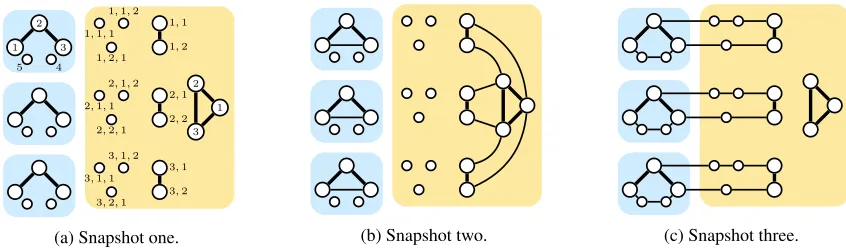
Figure 1: Illustration of the reduction from EXACT(3,4)-SAT to 2-SW TEMP. 2-COLORING of the proof of Theorem 4.2. Vertices and edges in the yellow shaded areas (right) correspond to a clause gadget for clause(x1∨x2∨x3). Vertices and edges
in the blue shaded areas (left) correspond to the variable gadgets forx1,x2, andx3. Thick edges appear in every snapshot while
thin edges only appear in one snapshot. In the first snapshot (a), the superscripts of the vertices used in the proof of Theorem 4.2 are shown. To keep the figure clean, those are omitted in the illustrations for snapshots two (b) and three (c).
tension and the auxiliary vertices arbitrarily. It is not hard to see that now the first∆-window is properly colored.
Lastly, we show how to color the third snapshot. Note that for the variable gadgets, the coloring in snapshot two deter-mines (up to switching the colors) how to color the variable gadgets in the third snapshot. This also determines how to color the auxiliary vertices and the extension of the core in the third snapshot. This potentially leaves edges of the ex-tension monochromatic. Note that in the second snapshot, all extension edges are properly colored except the one which, in the third snapshot, is connected to a variable that, in the given assignment, satisfies the clause. It is straightforward to check that in this case, this particular extension edge is prop-erly colored in the third snapshot. Lastly, the core is colored in a way that ensures that the edge that is colored monochro-matic in the second snapshot is colored properly in the third snapshot. It is easy to check that now the second∆-window is also properly colored.
(⇐): Assume we are given a proper sliding 2-window temporal 2-coloring for (G, λ). Then we construct a sat-isfying assignment for φ in the following way: Note that in the second snapshot each variable gadget contains a triangle with exactly one monochromatic edge. The edge {v(1)xi , v
(3)
xi } only exists in the second snapshot and hence is colored properly by any proper sliding 2-window tempo-ral 2-coloring. This means that either edge{vx(1)i , v
(2)
xi } or edge{v(2)xi, v
(3)
xi }is colored monochromatic. If{v
(1)
xi , v
(2)
xi } is colored monochromatic then we setxito true, otherwise we setxi to false. We claim that this yields a satisfying as-signment forφ. Assume for contradiction that it is not. Then there is a clausecjthat is not satisfied. Without loss of gener-ality, letx1,x2, andx3be the variables appearing incj. Then in the third snapshot, the clause gadget ofcjis connected to the variable gadgets ofx1,x2, andx3. It is easy to check
that in any proper sliding 2-window temporal 2-coloring, exactly one edge of the extension of any clause gadget is colored monochromatic in the second snapshot, hence this is also the case in the clause gadget ofcj. Without loss of
generality, let the monochromatically colored (in the second snapshot) extension edge of the clause gadget ofcjbe con-nected to the variable gadget ofx1in the third snapshot. It
is easy to check that for the sliding window temporal 2-coloring to be proper, the edge of the variable gadget ofx1
that is connected to the clause gadget ofcjin the third snap-shot needs to be colored properly in the second snapsnap-shot. By construction of(G, λ)this is a contradiction tocjnot being satisfied by the constructed assignment.
With small modifications to the reduction we get that SW-TEMP. COLORINGremains hard under the following restric-tions on the snapshots.
Corollary 4.3. SW-TEMP. COLORING is NP-hard for all k≥2,∆≥c, andT ≥∆ + 1for some constantceven if
• every snapshot is a cluster graph, or
• every snapshot has a dominating set of size one.
The reduction presented in the proof of Theorem 4.2 also yields a running time lower bound assuming the Exponen-tial Time Hypothesis (ETH) (Impagliazzo and Paturi 2001; Impagliazzo, Paturi, and Zane 2001).
Corollary 4.4. SW-TEMP. COLORING does not admit a ko(n)·f(T+k)-time algorithm for any computable functionf
unless ETH fails.
Proof. First, note that any 3SAT formula withmclauses can be transformed into an equisatisfiable EXACT (3,4)-SAT formula with O(m) clauses (Tovey 1984). The reduction presented in the proof of Theorem 4.2 produces an instance of SW-TEMP. COLORINGwithn=O(m)vertices,k= 2, andT = 3. Hence an algorithm for SW-TEMP. COLORING
with running timeko(n)·f(T+k)for some computable
func-tionfwould imply the existence of an2o(m)-time algorithm
for 3SAT. This is a contradiction to ETH.
Optimal Exponential-Time Algorithm Assuming ETH.
In the following we give an exponential-time algorithm for
the ETH. The main idea is to enumerate all partial proper sliding∆-window temporal colorings for time windows of size 2∆and then check whether we can combine them to a proper sliding∆-window temporal coloring for the whole temporal graph.
Theorem 4.5. SW-TEMP. COLORING can be solved in O(k4∆·n·T)time.
Proof. For the sake of simplicity, we assume thatT is divis-ible by∆. The general case can be proven alike. We give the following algorithm for the problem:
1. For 2∆-windows Wi = [i∆ + 1,(i+ 2)∆] for i ∈
{0,1, . . . , T /∆−2}, enumerate all partial proper slid-ing∆-window temporal coloringsφWi, where each trivial snapshot is colored in some fixed but arbitrary way1. 2. Create adirected acyclic graph(DAG) withφWi as
ver-tices and connectφWi andφWi+1 with a directed arc if
the two proper∆-temporal colorings agree on the over-lapping part.
3. Create a source vertexsand connect it to allφW1 with
a directed arc and we create a sink vertex t and add a directed arc from allφWT /∆−2 to it.
4. If there is a path fromstot, answer YES, otherwise NO. The running time is dominated by checking whethersandt are connected in the last step of the algorithm. This can be done e.g. by a BFS on the constructed DAG. The DAG has at mostk2∆·n·Tvertices and at mostk4∆·n·Tedges.
Fixed-Parameter Tractability. Next, we show how to ex-tend the algorithm presented in Theorem 4.5 to achieve lin-ear time fixed-parameter tractability with respect to the num-bernof vertices. The main idea is to reduce the number of non-trivial snapshots in each∆-window.
Theorem 4.6. SW-TEMP. COLORING can be solved in O(T)time ifnis a constant.
Proof. We present a preprocessing step to reduce the num-ber of non-trivial snapshots in any∆-window and then use the algorithm of Theorem 4.5 to solve the problem.
The reduction rule is based on the observation that if some snapshot appears at leastn2times in a∆-window, then the edges of this snapshot can be properly colored with 2 col-ors within the∆-window. In other words, all butn2 copies of the snapshot in the∆-window are redundant for optimal coloring and each of them could be replaced by the trivial snapshot. When implementing this idea one should take care to guarantee that replacing a snapshot by the trivial one does not reduce the number of copies of the snapshot in other∆ -windows which contain at mostn2copies of the snapshot.
Formally the reduction rule is as follows. Since the num-ber of different snapshots is at most2(n2) ≤2n2, by the
pi-geonhole principle if ∆ > 2·2n2 ·n2, then in every ∆ -window there exists a snapshot that appears more than2n2
times in that∆-window. For every such a snapshot that con-tains at least one edge, we replace by the trivial snapshot one of its ”middle” copies, that is, one that has at leastn2
1
This is an important trick that allows us to use this algorithm for the FPT result in Theorem 4.6.
copies appearing earlier and n2 copies that appear later in the∆-window. This reduction rule guarantees that every∆ -window that contains the modified snapshot also contains at leastn2 copies of the original snapshot appearing either
earlier or later in the∆-window.
The reduction rule can be applied exhaustively by linearly sweeping over all ∆-windows once in the following way. For each different graph (snapshot) we store a list of occur-rences and update these lists every time we move the ∆ -window by one. Having these lists, it is straightforward to count the occurrences and replace the middle ones by triv-ial snapshots. When we move the∆-window, we just have to update two lists: the one of the graph that enters the∆ -window and the one of the graph that leaves. This requires a lookup table of size2(n2)≤2n2 but takes only linear time
inT. Note that after this procedure, every∆-window con-tains at most2·2n2·n2non-trivial snapshots.
Now we apply the algorithm of Theorem 4.5. Note that after the reduction step the number ofnon-trivialsnapshots in every∆-window depends only onn. Furthermore, since we can assume thatk ≤ n, the number of colorings that are enumerated in Step 1 of the algorithm in Theorem 4.5 is bounded by a function ofn. This completes the proof.
The FPT result of Theorem 4.6 is complemented by the following theorem, in which we exclude the possibility of a polynomial-sized kernel for SW-TEMP. COLORINGwith respect to the numbernof vertices. This comes in contrast to the existence of a polynomial-sized kernel for TEMPORAL
COLORINGwith respect ton(cf. Theorem 3.3).
Proposition 4.7. SW-TEMP. COLORINGdoes not admit a polynomial-sized kernel with respect to the numbernof ver-tices for all∆≥2andk≥2unless NP⊆coNP/poly.
Structural Graph Parameters and Approximation. Fi-nally, we investigate the possibility to structurally improve the fixed-parameter tractability result by replacing the pa-rameternwith a smaller parameter. We answer this nega-tively by showing that∆-SW-TEMP.k-COLORINGremains NP-hard even if the underlying graph has a constant-size vertex cover, which is a fairly large structural parameter.
Theorem 4.8. Letk≥2. Then 2-SW-TEMP.k-COLORING
is NP-hard, even if the vertex cover number of the underlying graph is at most2k+ 13.
Next, we consider a canonical optimization version of SW-TEMP. COLORING, which we call MINIMUM SW-TEMP. COLORING, where the goal is to minimize the num-ber of colors k. Using Theorem 4.6, we provide an FPT-approximation algorithm with an additive error of one where the parameter is the vertex cover number of the underlying graph. Considering that we cannot hope for an exact FPT algorithm for parameter “vertex cover number of the under-lying graph” unless P =NP (cf. Theorem 4.8), this is the best we can get from a classification standpoint.
References
Aaron, E.; Krizanc, D.; and Meyerson, E. 2014. DMVP: foremost waypoint coverage of time-varying graphs. InWG 2014, 29–41.
Akrida, E. C.; Gasieniec, L.; Mertzios, G. B.; and Spirakis, P. G. 2016. Ephemeral networks with random availability of links: The case of fast networks.J. Parallel Distrib. Comput. 87:109–120.
Akrida, E. C.; Gasieniec, L.; Mertzios, G. B.; and Spirakis, P. G. 2017. The complexity of optimal design of temporally connected graphs.Theory Comput. Syst.61(3):907–944.
Akrida, E. C.; Mertzios, G. B.; Spirakis, P. G.; and Zama-raev, V. 2018. Temporal vertex covers and sliding time win-dows. InICALP 2018, 148:1–148:14.
Bentert, M.; Himmel, A.-S.; Molter, H.; Morik, M.; Nieder-meier, R.; and Saitenmacher, R. 2018. Listing all maximal k-plexes in temporal graphs. InASONAM 2018, 41–46.
Bui-Xuan, B.-M.; Ferreira, A.; and Jarry, A. 2003. Com-puting shortest, fastest, and foremost journeys in dynamic networks. Int. J. Found. Comput. Sci.14(2):267–285.
Casteigts, A., and Flocchini, P. 2013a. Deterministic Algo-rithms in Dynamic Networks: Formal Models and Metrics. Technical report, Defence R&D Canada.
Casteigts, A., and Flocchini, P. 2013b. Deterministic Algo-rithms in Dynamic Networks: Problems, Analysis, and Al-gorithmic Tools. Technical report, Defence R&D Canada.
Casteigts, A.; Flocchini, P.; Quattrociocchi, W.; and San-toro, N. 2012. Time-varying graphs and dynamic networks. IJPEDS27(5):387–408.
Chen, J.; Molter, H.; Sorge, M.; and Such´y, O. 2018. Cluster editing in multi-layer and temporal graphs. InISAAC 2018. To appear.
Clementi, A. E. F.; Macci, C.; Monti, A.; Pasquale, F.; and Silvestri, R. 2010. Flooding time of edge-markovian evolv-ing graphs. SIAM J. Discr. Math.24(4):1694–1712.
Cygan, M.; Fomin, F. V.; Kowalik, Ł.; Lokshtanov, D.; Marx, D.; Pilipczuk, M.; Pilipczuk, M.; and Saurabh, S. 2015.Parameterized Algorithms. Springer.
Enright, J.; Meeks, K.; Mertzios, G. B.; and Zamaraev, V. 2018. Deleting edges to restrict the size of an epidemic in temporal networks. CoRRabs/1805.06836.
Erlebach, T.; Hoffmann, M.; and Kammer, F. 2015. On temporal graph exploration. InICALP 2015, 444–455.
Ferreira, A. 2004. Building a reference combinatorial model for MANETs.IEEE Network18(5):24–29.
Flocchini, P.; Mans, B.; and Santoro, N. 2009. Exploration of periodically varying graphs. InISAAC 2009, 534–543.
Fluschnik, T.; Molter, H.; Niedermeier, R.; and Zschoche, P. 2018. Temporal graph classes: A view through temporal separators. InWG 2018, 216–227.
Ghosal, S., and Ghosh, S. C. 2015. Channel assignment in mobile networks based on geometric prediction and random coloring. InLCN 2015, 237–240.
Giakkoupis, G.; Sauerwald, T.; and Stauffer, A. 2014. Ran-domized rumor spreading in dynamic graphs. In ICALP 2014, 495–507.
Himmel, A.; Molter, H.; Niedermeier, R.; and Sorge, M. 2017. Adapting the bron-kerbosch algorithm for enumer-ating maximal cliques in temporal graphs. Social Netw. Analys. Mining7(1):35:1–35:16.
Holme, P., and Saram¨aki, J., eds. 2013.Temporal Networks. Springer.
Impagliazzo, R., and Paturi, R. 2001. On the complexity of k-sat.J. Comput. Sys. Sci.62(2):367–375.
Impagliazzo, R.; Paturi, R.; and Zane, F. 2001. Which prob-lems have strongly exponential complexity?J. Comput. Sys. Sci.63(4):512–530.
Kempe, D.; Kleinberg, J.; and Kumar, A. 2002. Connectivity and inference problems for temporal networks. J. Comput. Sys. Sci.64(4):820–842.
Latapy, M.; Viard, T.; and Magnien, C. 2018. Stream graphs and link streams for the modeling of interactions over time. Social Netw. Analys. Mining8(1):61:1–61:29.
Leskovec, J.; Kleinberg, J. M.; and Faloutsos, C. 2007. Graph evolution: Densification and shrinking diameters. TKDD1(1).
Mertzios, G. B.; Michail, O.; Chatzigiannakis, I.; and Spi-rakis, P. G. 2013. Temporal network optimization subject to connectivity constraints. InICALP 2013, 657–668.
Mertzios, G. B.; Molter, H.; and Zamaraev, V. 2018. Sliding window temporal graph coloring.CoRRabs/1811.04753. Michail, O., and Spirakis, P. G. 2016. Traveling salesman problems in temporal graphs.Theor. Comput. Sci.634:1–23. Michail, O., and Spirakis, P. G. 2018. Elements of the theory of dynamic networks.Comm. ACM61(2):72–72.
Michail, O. 2016. An introduction to temporal graphs: An algorithmic perspective.Internet Math.12(4):239–280. Tang, J. K.; Musolesi, M.; Mascolo, C.; and Latora, V. 2010. Characterising temporal distance and reachability in mobile and online social networks. Computer Communication Re-view40(1):118–124.
Tovey, C. A. 1984. A simplified NP-complete satisfiability problem.Discrete Appl. Math.8(1):85–89.
Viard, T.; Latapy, M.; and Magnien, C. 2016. Comput-ing maximal cliques in link streams. Theor. Comput. Sci. 609:245–252.