The Thirty-Third AAAI Conference on Artificial Intelligence (AAAI-19)
Compiling Bayesian Network Classifiers into Decision Graphs
Andy Shih, Arthur Choi, Adnan Darwiche
Computer Science DepartmentUniversity of California, Los Angeles {andyshih,aychoi,darwiche}@cs.ucla.edu
Abstract
We propose an algorithm for compiling Bayesian network classifiers into decision graphs that mimic the input and output behavior of the classifiers. In particular, we compile Bayesian network classifiers into ordereddecision graphs,
which are tractable and can be exponentially smaller in size than decision trees. This tractability facilitates reasoning about the behavior of Bayesian network classifiers, including the explanation of decisions they make. Our compilation al-gorithm comes with guarantees on the time of compilation and the size of compiled decision graphs. We apply our com-pilation algorithm to classifiers from the literature and discuss some case studies in which we show how to automatically ex-plain their decisions and verify properties of their behavior.
1
Introduction
Bayesian network classifiers have been used extensively in the literature (Friedman, Geiger, and Goldszmidt 1997; Ng and Jordan 2002; Pernkopf and Bilmes 2005; Roos et al. 2005). These classifiers encode a probability distribution over a set of features and a class variable, and then classify an observation on features based on the posterior marginal of the class variable. Although the classification process com-putes probabilities, the classifier’s behavior can be captured as a discrete mapping from the states of features (instances) to the states of the class variable (classes). We refer to this mapping as the classifier’sdecision function.Obtaining the decision function in a symbolic, tractable form was recently shown to be useful for explaining the decisions and formally verifying the properties of classifiers (Shih, Choi, and Dar-wiche 2018a; 2018b).
Previous work proposed algorithms for compiling Naive Bayes and latent tree classifiers into decision graphs (Chan and Darwiche 2003; Shih, Choi, and Darwiche 2018b). In this paper, we propose an algorithm that compiles a Bayesian network classifier with an arbitrary structure. We then illustrate the utility of our compilation algorithm through case studies, in which we symbolically reason about the behavior of some Bayesian network classifiers from the literature. This follows a recent trend in analyzing machine learning models using symbolic approaches (Narodytska et al. 2018; Katz et al. 2017).
Copyright c2019, Association for the Advancement of Artificial Intelligence (www.aaai.org). All rights reserved.
In particular, our algorithm compiles a Bayesian net-work classifier into anordered decision graph,a well-known and tractable class of decision graphs in which features are tested in the same order, along each path from the root of the graph to any of its leaves. When the features and the class variable are binary, the ordered decision graph is known in the literature as anOrdered Binary Decision Di-agram (OBDD)(Bryant 1986; Meinel and Theobald 1998; Wegener 2000). When only the class variable is binary, it is known as anOrdered Decision Diagram (ODD)(Chan and Darwiche 2003). In this paper, we focus on the case of bi-nary classifiers, but discuss an adaptation of our proposed compilation algorithm to support multi-class classifiers.
This paper is structured as follows. Section 2 provides an introduction to Bayesian network classifiers and ODDs. Sections 3 and 4 provide key results on Bayesian network classifiers, which are utilized by our compilation algorithm in Section 5. Experimental results relating to scalability are then given in Section 6, followed by a case study in Sec-tion 7. We finally conclude in SecSec-tion 8.
2
Background
In this section, we describe Bayesian network classifiers and Ordered Decision Diagrams in more detail.
Bayesian Network Classifiers
ABayesian network classifier is a Bayesian network con-taining a special set of variables: a single classvariableC
andnfeature variablesX = {X1, . . . , Xn}. The classC is usually a root in the network and the featuresXare usu-ally leaves. An instantiation of variablesXis denotedxand called aninstance.When the class variable is binary, its two values c and¯c correspond to 1 and 0 decisions. A binary
Bayesian network classifier specifying probability distribu-tionPr(.)will classify an instancexas 1 iffPr(c|x)≥T,
whereTis called the classificationthreshold.We denote the decision function of a classifierBasFB.
Ordered Decision Diagrams
C
A N1
G F M
N2
(a) Bayesian network classifier
0 1
A
F G
F
M
(b) Ordered Decision Diagram
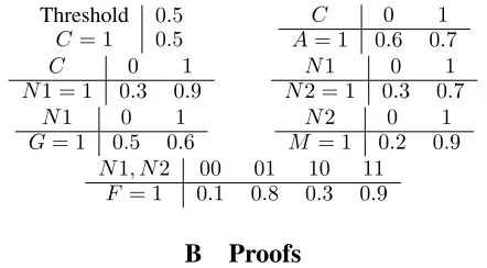
Figure 1: A Bayesian network classifier and its correspond-ing decision graph. The details of the Bayesian network clas-sifier are provided in Table 3 in the Appendix.
graph with two sinks called the 1-sink and 0-sink. Every node (except the sinks) in the OBDD is labeled with a vari-ableXiand has two labeled outgoing edges: the1-edge and the0-edge. The labeling of the OBDD nodes respects some global ordering of the variablesX: if there is an edge from a node labeledXito a node labeledXj, thenXimust come beforeXj in the global ordering. To evaluate the OBDD on an instance x, start at the root node of the OBDD and let
xi be the label of the current node. Repeatedly follow the
xi-edge of the current node, until a sink node is reached. Reaching the1-sink meansxis evaluated to 1 and reaching the0-sink meansxis evaluated to 0 by the OBDD.
An OBDD is defined over binary variables, but can be extended to discrete variables with arbitrary values. This is called an ODD: a node labeled with variable Xi has one outgoing edge for each value of variable Xi. Hence, an OBDD/ODD can be viewed as representing a functionf(X) that maps instancesxinto{0,1}.
Consider the Bayesian network classifier in Figure 1a, which classifies a movie as being a box office success or not. It has four binary features:A(Adapted Screenplay),G
(Great Cinematography),F (Famous Cast), andM
(Mar-keting). The ODD in Figure 1b captures the input and output behavior of the classifier in a tractable form. That is, given an instantiation of the features{A,G,F,M}, we start from the root node of the ODD and repeatedly follow the solid edge if the feature of the current node is set to 1, and follow the dotted edge otherwise. We will reach either the 0-sink or the 1-sink, which tells us if the instance is classified as 0 or 1. Moreover, the reached decision is guaranteed to match the one obtained from the Bayesian network classifier in Fig-ure 1a. Given this tractable representation, we follow the ap-proach of (Shih, Choi, and Darwiche 2018b) to efficiently explain the decisions of the Bayesian network classifier.
Consider a movie that is an adapted screenplay, has great cinematography, a famous cast, heavy marketing, and is classified as being a box office success. This movie corre-sponds to features{A=1,G=1,F=1,M=1}and a
classifica-tion of 1. Using the ODD in Figure 1b we can deduce, in time linear on the size of the ODD, that the movie could have had poor cinematography and low marketing, and would still be classified as being a box office success. In fact, the
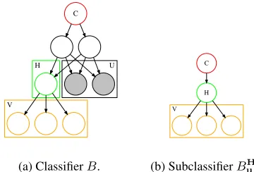
par-H U
V
C
(a) ClassifierB.
V C
H
(b) SubclassifierBH u. Figure 2: Variable H splits features into (U,V). When given an instantiation uon the variables U, we can con-struct a subclassifier that has the same decision function as the original classifier over variablesV.
tial instantiation{A=1,F=1}completely determines that the
movie will be classified as being successful, regardless of how the remaining features are set. Furthermore, we can for-mally verify that the classifier is monotonic. That is, any in-stance classified as 1 remains classified as 1 even if some of its features are flipped from 0 to 1.
The above analysis is exemplary of many more queries that one can efficiently answer about a Bayesian network classifier, once it has been compiled into an ODD. We de-scribe below some more queries that can also be efficiently answered (Shih, Choi, and Darwiche 2018a).
• Robustness: Given an instance, what is the least number of features we need to flip to change its classification? • Irrelevant Features: Are there features that do not impact
any classification?
• If-Then Rules: Does the classifier satisfy some given rules of thumb?
The above queries can be computed in linear or quadratic time in the size of the compiled ODD. This highlights the significance of compiling Bayesian network classifiers into ODDs. Next, we present some key observations about Bayesian network classifiers that we exploit later.
3
Subclassifiers
Our compilation algorithm is based on recursively decom-posing into smaller classifiers and identifying those that are equivalent to avoid the compilation of a classifier if an equiv-alent one has already been compiled. In this section we present the method of decomposing into smaller classifiers, which can be described at a high level as follows. Given a Bayesian network classifierB, letUandVbe a partition of its featuresXand letHbe a variable not inX. Suppose now
that we are only interested in classifying instancesxthat set featuresU to some stateu. When certain conditions hold, we can perform the classification using asmallerclassifier, which is obtained from classifierBas follows:
– NodeH is disconnected from its parents andC, the class
– A CPT is assigned toHbased on inference onB.
– A prior is assigned toCbased on inference onB.
– Leaves are repeatedly removed from classifierBas long
as they are not inC∪H∪V.
The resulting classifier is called asubclassifier.Figure 2 de-picts an example of the structural changes needed to con-struct a subclassifier. The main insight regarding these sub-classifiers is that they compute the same decision function over the remaining variables V as the original classifier. Once we fixuand obtain a subclassifierBH
u from an orig-inal classifierB, the decision functionFBH
u(v)will output the same classification asFB(uv). This key property will be used in the algorithm to reduce the compilation of a classi-fier into the compilation of subclassiclassi-fiers.
We will now spell out the above result on subclassifiers. We first state the conditions under which a subclassifier can be constructed.
Definition 1 Let(U,V)be a partition of the featuresXin a Bayesian network classifierB, and letH be a variable outsideX. We say thatH splitsfeaturesXinto(U,V)iff
Hd-separates featuresVfromCandU.
Recall thatZd-separatesXfromYifXandYare in-dependent givenZ(Darwiche 2009). We are now ready to define subclassifiers.
Definition 2 LetB be a Bayesian network classifier,H be a variable that splits features into(U,V), andube an in-stantiation of features U. Thesubclassifier for H and u, denotedBH
u, is obtained from classifierBas follows: 1. Disconnect nodeHfrom its parents.
2. MakeH a child of class variableC, and set its Condi-tional Probability Table (CPT) toP(H|Cu).
3. Set the CPT ofCtoP(C|u).
4. Repeatedly remove every leaf node fromBthat is not in
C∪H∪V.
Constructing a subclassifier requires some computational work on the original classifierB. First, we need to identify
a variableHthat satisfies the condition of Definition 1. This
can be done in polynomial time as it only involves reason-ing about d-separation (Darwiche 2009). Second, we need to determine the CPTs ofH andC, which require the
com-putation of posteriors on theH andC, given the stateuof featuresU. This requires exact inference on the classifierB.
We will later provide a bound on the number of inference calls made by our compilation algorithm for this purpose. The next theorem formalizes the property of subclassifiers. Theorem 1 LetBbe a Bayesian network classifier and let
H be a variable that splits features into(U,V). For a sub-classifierBH
u, we haveFB(uv) =FBH
u(v)for all instanti-ationsvof featuresV.
According to this theorem, the classification of an instance uvby classifierBwill match the classification ofvby sub-classifierBHu. As we shall see, when our compilation
algo-rithm fixes the state of featuresUtou, it will construct and recursively compile the subclassifierBuH.
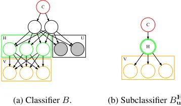
H U
V
C
(a) ClassifierB.
V C
H
(b) SubclassifierBH u. Figure 3: A construction of a subclassifier using a set of splitting nodesH.
Multiple Splitting Nodes
For Bayesian network classifiers with dense structure, there may not exist a single node H that splits the features into
two parts. In such cases, we can actually relax the splitting node to the case of a set of nodes, using the formulation of a meganode (Russell and Norvig 2016). More specifically, a set of nodes in a Bayesian network can sometimes be re-placed by a single meganode whose state space is the Carte-sian product of the state spaces of the set of nodes (Figure 3). To simplify the discussion, for the rest of the paper we will only focus on the case whereHis a single node.
4
Equivalent Classifiers
We will now introduce the second key result that will form the basis of our algorithm for compiling a Bayesian network classifier into an ODD. This result provides a method for de-tecting when two “similar” Bayesian network classifiers in-duce the same decision function. In this section we assume, without loss of generality, that the classifier has a class node
C which has a single childH. This assumption is satisfied
by all subclassifiers and can easily be satisfied for any clas-sifier by adding a dummy class node with the original class node as its single child. First we define when two classifiers are considered similar.
Definition 3 LetBbe a Bayesian network classifier with a class node C which has a single child nodeH. A second Bayesian network classifier issimilartoBif it has the same structure asBand differs only in the CPTs ofCandH.
LetX be the feature variables of two similar classifiers
B andB0. Note that P(X|H)is the same across the two classifiers, andH d-separatesCfromXby our earlier as-sumption. Thus, we can rewriteP(C|X)as follows:
P(C|x) =X h
P(C|h)P(h|x)
=X h
P(C, h)P(x|h)/P(x) (1)
So far, the results from Section 3 and this section have not assumed that the class variableCand the variableHare
α γ β
Figure 4: Visualization of the equivalence interval of a clas-sifierB. The red dots represent instances classified as1and the blue dots represent instances classified as0. A classifier that is similar toBshares the same decision function asB
if its coefficientγfalls within the equivalence interval ofB,
depicted by the white region betweenαandβ.
section, we will assume that nodesCandHare binary, and
the classification threshold ist. In this setting, we have an
efficient way of detecting when two similar classifiers share the same decision function, in time linear in the number of featuresX. We present the details next.
Settingah=P(c, H=h)−tP(H =h), we can rewrite the classification as a linear inequality.
X
h
P(c, h)P(x|h)≥tP(x) X
h
(P(c, h)−tP(h))P(x|h)≥0 X
h
ahP(x|h)≥0 (2) For two similar classifiers, the valuesahvary butP(x|h) is the same. To detect if two similar classifiers share the same decision function, we just need to verify that the two sets of valuesahclassify all instancesxthe same way. To do so, we define the sign, margin, and coefficient of such classifiers. Definition 4 LetBbe a non-trivial1Bayesian network clas-sifier with a thresholdtand a binary class nodeCwhich has a single binary child nodeH. Letσdenote thesignof the classifier, which is defined to be 1 ifP(c|H = 1)≥tand 0 otherwise. Themarginα, βandcoefficientγ ofB are de-fined as follows:
α = max
x:FB(x)=1
P(x|H = 1−σ)/P(x|H =σ)
β = min
x:FB(x)=0
P(x|H = 1−σ)/P(x|H =σ)
γ = −1· P(c, H=σ)−tP(H =σ)
P(c, H= 1−σ)−tP(H = 1−σ) That is,αis the largest value ofP(x|H= 1−σ)/P(x|H =
σ)attained by any instance classified as1, andβis the
small-est such value attained by any instance classified as0 (see Figure 4). The valuesα,β, and γcome from a
rearrange-ment of Equation 2 for the case of a binaryHvariable. The
notion of a margin was actually identified by (Chan and Dar-wiche 2003) in connection to Naive Bayes classifiers, and turns out to apply to general Bayesian network classifiers.
The next result was proven only for Naive Bayes clas-sifiers in (Chan and Darwiche 2003). Our generalization is phrased differently and is more succinct.
1A non-trivial classifier with a binary class node classifies at
least one instance as 1 and at least one instance as 0.
Theorem 2 LetBbe a non-trivial Bayesian network clas-sifier with a binary class nodeCand a single binary child nodeH. LetB0be a second classifier that is similar toBand
has the same sign asB. Lettbe their threshold,(α, β)be the margin of classifierB, andγbe the coefficient ofB0. The two classifiers have the same decision function,FB =FB0,
iffγbelongs to the interval[α, β). This is called the equiva-lence interval of classifierB.
The above theorem enables us to perform binary search over equivalence intervals to identify equivalent subclassi-fiers: ones that lead to the same decision function and hence the same compilation. This technique avoids the compila-tion of a subclassifier if an equivalent one has already been compiled.
5
From Numeric Bayesian Network
Classifiers to Symbolic ODDs
We now present our algorithm for compiling a Bayesian net-work classifierB into an ODD. We address the case of
bi-nary classifiers first and then describe the adaptation of our algorithm to multi-class classifiers.
The overall structure of the algorithm is pretty simple. We first identify a binary variableH that splits the features into
(U,V). We then start enumerating over the values of fea-tures inUas if we are building a decision tree (in a depth-first manner). Each leaf of this decision tree corresponds to a distinct instantiationuand a subclassifierBuH with its
equivalence interval. These subclassifiers are similar to one another, since they differ only in the CPTs of class Cand
variableH. Our algorithm will then compile these
subclas-sifiers recursively using the same technique, except that it will avoid compiling a subclassifier if it already compiled an equivalent one—as determined by Theorem 2.
The efficiency of this algorithm depends on the choice of variableH and the corresponding feature decomposition
(U,V)as we wantUto be as small as possible. We identify such feature decompositions in a preprocessing step. That is, after first decomposing features into (U,V), using an
ap-propriateH, we follow by decomposingVrecursively. This leads us to the notion of ablock orderingof features. Definition 5 Given a Bayesian network classifier, a block
orderingof its featuresXis a sequenceπ= (X1, . . . ,Xm)
such thatX1, . . . ,Xmis a partition of featuresX, and for each0< k < m, there exists a binary variableHthat splits featuresXinto(X1∪. . .∪Xk,Xk+1∪. . .∪Xm). Each elementXiis called ablockof the block orderingπ. We will assume that the features in a block are ordered (ar-bitrarily). As such, we will refer to features by their position in the block orderingπ.
We will later discuss a heuristic for obtaining a block or-der, which we used in our experiments. But for now, we will discuss Algorithms 1 and 2. Algorithm 1 is passed a Bayesian network classifierBand a block orderingπof
Algorithm 1compile-classifier(B, π)
input:Bayesian network classifierBand block orderingπof
fea-tures
output:ODD for the decision function of classifierB
main:
1: 0-sink ←terminal ODD node labeled with0
2: 1-sink ←terminal ODD node labeled with1
3: D←compile-subclassifier(B,{}, π,0)
4: return reduced form ofD
Algorithm 2compile-subclassifier(B,u, π, k)
input:Bayesian network classifierB, instantiationuof some
fea-tures, block orderingπof features, integerk
output:ODD for the decision function of classifierB
main:
1: ifuis an instantiation of a block in orderingπthen
2: B←get-subclassifier(B,u, π, k)
3: ifBhas no feature variablesthen
4: return get-sink(B)
5: γ, σ←coefficient and sign ofB
6: D←find-in-cache(γ, σ, k)
7: ifD=nullthen
8: D←compile-subclassifier(B,{}, π, k)
9: I←equivalence-interval(D)
10: store-in-cache(D, I, σ, k)
11: return D
12: X←feature at positionkin orderingπ
13: S← {}
14: foreach statexof feature Xdo
15: C←compile-subclassifier(N,u∪x, π, k+ 1)
16: add(C, x)to setS
17: return get-odd-node(S)
interval,σis a boolean, andkis an integer. Such a cache
en-try means that ODDDis the result of compiling a
subclas-sifierButhat has equivalence intervalIand signσ. It also means that the last feature in blockUis at positionk−1in the block orderingπ. The cache is fetched based on a
coef-ficientγ, a signσand a levelk. That is, it returns ODDDif γ∈Ifor the sameσand samek.
Algorithm 2 makes use of four auxiliary functions. First,
get-subclassifier(B,u, π, k) constructs a
subclassi-fier and requires a constant number of calls to an exact in-ference algorithm to get the coefficients of the subclassifier.
get-sink(B) takes in a subclassifier with no more
fea-tures, and returns either the0-sinkor the1-sinkbased
on a simple check.equivalence-interval(D)
com-putes the equivalence interval of the classifier leading to ODDD. This is done in constant time using the equivalence
intervals for the children ofD(Chan and Darwiche 2003).
Finally,get-odd-node(S) returns an ODD node, which
is defined by the setSthat specifies the node’s children and
the labels of edges pointing to these children.
Algorithm 3 implements a simple, greedy heuristic for obtaining a block ordering of features. Its running time is
O(n4), wherenis the number of features, which was suffi-cient for our experiments.
Algorithm 3block-order(B,X)
input:A Bayesian network classifierBwith featuresX
output:A block orderingπof the featuresX
main:
1: H,U,V←class variable ofB,X,∅
2: foreach variableH0that splits featuresXinto(U0,V0)do
3: if|U0| ≤ |U|then
4: H,U,V←H0,U0,V0
5: u←some instantiation ofU
6: return U,block-order(BHu,V)
H0
H2
X0 X1
H4 X3
X2
...
X2n-2 X2n X2n-1
(a) Ladder classifier (vari-ablesXiare features)
H0
(b) Cluster classifier (clouds contain arbitrary structure)
Figure 5: Examples of classifier families with improved compilation time.
We close this section by providing time and size bounds on our compilation algorithm. We later show that for certain classes of Bayesian networks, these bounds can be as tight as the bounds provided by (Chan and Darwiche 2003) for compiling Naive Bayes classifiers into ODDs.
Definition 6 Letπ= (X1, . . . ,Xm)be a block ordering of the features in a Bayesian network classifierB. Letpidenote the size of the state space of the features in blocki, and let
s(i, j) = log2(pi×. . .×pj). Thewidthwπof this order and
thecompilation widthwBof classifierBare defined as:
wπ = max
i∈{1,...,m}
pi·min(s(1, i−1), s(i, m)
]
wB = min π wπ.
We now have the following bounds on Algorithm 1. Theorem 3 The number of nodes in the ODD returned by Algorithm 1 isO(2wπ), wherew
π is the width of orderπ. Moreover, the running time of the algorithm is O(P T +
wπ2wπ), wherePis the sum of the state space sizes of blocks inπandTis the time of an inference call on the classifier.
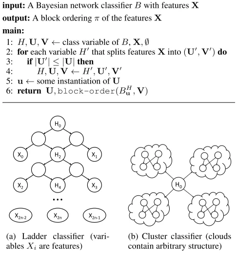
Consider the family of ladder classifiers depicted in Fig-ure 5a, which hasn= 2m+ 1features. We can use the se-quence of nodesH2, H4, . . . , H2mto decompose features, leading to the block ordering
[X0, X1],[X2, X3], . . . ,[X2m−2, X2m−1, X2m],
The family of cluster classifiers in Figure 5b has similar bounds. Assume that we havenfeatures andkclusters, with
each cluster havingn/kfeatures. We can repeatedly use the
nodeH0to split features intokblocks of sizen/k, leading to a block order widthn/2, assuming binary features, and a largest block sizen/k. The size of the ODD isO(2n/2)and the running time isO(k2n/kT +n2n/2).
What is interesting about these bounds is that they match the ones for compiling Naive Bayes classifiers to ODDs (Chan and Darwiche 2003)—an NP-hard problem as shown by (Shih, Choi, and Darwiche 2018b). In practice, however, the time and size complexity of Algorithm 1 can be signifi-cantly better as we show in Section 6.
Multi-class Classifiers
We can adjust our algorithm to support the compilation of multi-class classifiers. For a multi-class classifierB, an
in-stance is classified based on the highest posterior probabil-ity among all states of the class variable. That is,FB(x) = argmaxcP(c|x). Since the output is non-binary, we use a
variation of the ODD called the Algebraic Decision Diagram (ADD), which has multiple sinks, one for each state of the class node (Bahar et al. 1997). ADDs are tractable, so we can still explain and perform verification on the behavior of multi-class classifiers efficiently.
The construction of a subclassifier in Section 3 general-izes directly to multi-class classifiers. Equation 1 holds for multi-class classifiers as well. Our current formulation of equivalence intervals is designed for binary classifiers, so for future work we will look into generalizing equivalence intervals to multi-class classifiers.
We can still obtain a bound on the compilation time using a naive method of detecting equivalent subclassifiers. First, we modify Algorithm 1 to support multiple sinks. We mod-ify Algorithm 2 so that instead of finding an equivalent sub-classifier using binary search on equivalence intervals, we enumerate over all instances of the subclassifier if the num-ber of instances is small enough. Using Equation 1 to share inference calls among similar subclassifiers, we can get a bound on the running time of our adapted compilation algo-rithm on multi-class classifiers.
Theorem 4 The running time of the adapted version of Al-gorithm 1 on a multi-class Bayesian network classifier with a block orderingπisO(P T + 2s), whereP is the sum of the state space sizes of all blocks inπ,T is the time of an inference call on the classifier, andsis the log of the product of the state space sizes of blocks inπ.
Reducing the classifier into subclassifiers provides signif-icant savings on the number of exact inference calls. The number of computations may be greatly reduced once we develop equivalence intervals for multi-class classifiers.
6
Experiments
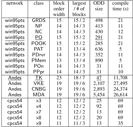
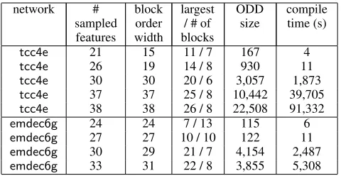
Table 1 summarizes compilation experiments we ran on three binary Bayesian networks using all leaf nodes as fea-tures. For each network we included a number of classi-fiers, each corresponding to one root of the network, using a
Table 1: win95pts has76 nodes,16features and width 9.
Andeshas223nodes,24features and width18.cpcs54has
54nodes,13features and width14. Width refers to the net-work tree-width, approximated by the minfill heuristic.
network class block order width
largest / # of blocks
ODD
size compiletime (s)
win95pts GRDS 15 15 / 2 498 21
win95pts NP 14 14 / 3 413 11
win95pts NC 14 14 / 3 430 12
win95pts PO 15 15 / 2 291 21
win95pts POOK 15 15 / 2 285 21
win95pts PAT 13 13 / 4 636 5
win95pts PDrvr 14 14 / 3 352 11
win95pts PMem 13 13 / 4 890 5
win95pts POn 14 14 / 3 31 11
win95pts PPpr 14 14 / 3 31 10
Andes TK 23 18 / 7 47 11,708
Andes VKE 19 19 / 6 2,107 27,495
Andes CNBG 19 19 / 6 2,893 24,374
Andes MDA 19 19 / 6 5,454 26,614
cpcs54 x3 12 12 / 2 25 69
cpcs54 x4 12 12 / 2 92 69
cpcs54 x7 12 12 / 2 13 69
cpcs54 x8 12 12 / 2 20 69
cpcs54 x9 11 11 / 3 13 35
threshold of1
2. Table 2 provides similar results on two other binary networks, except in this case we sampled some of the leaf nodes to include as features (the networks were too large to fully compile). Inference calls were performed using the SamIAm library.2
The actual sizes of the resulting ODDs are much smaller than the theoretical upper bounds. For example, the size of the ODD of the Andes classifier with root ValueKnownEq(VKE)is less than 1% of the bound given by the block order width. The limiting factor for the compi-lation algorithm is the compicompi-lation time, which depends on the treewidth of the network and scales exponentially with respect to the largest feature block. The treewidth affects the time of each inference call, and the largest feature block bounds the number of inference calls made by the compila-tion algorithm. For example, the twoemdec6gexperiments
in Table 2 with27and30features differ only by2in block order width. But, since they differ by11in the largest fea-ture block, we notice a large jump in the compilation time for these two experiments (two orders of magnitude). On the other hand, the experiment with30and33features also differ by2in block order width. Since their largest feature blocks differ only by 2, the compilation times are compa-rable (factor of2). The ODD size and compilation time are also significantly affected by the threshold of the classifier. A heavily biased threshold can lead to a very small ODD and a short compilation time, while a balanced threshold gener-ally leads to larger ODDs.
Our results suggest that the compilation algorithm can be used to implement and deploy Bayesian network classifiers
Table 2: Networktcc4ehas98nodes and width10. Network
emdec6ghas168nodes and width7. We uset27as the class
node fortcc4e, andx29as the class node foremdec6g.
network # sampled features
block order width
largest / # of blocks
ODD
size compiletime (s)
tcc4e 21 15 11 / 7 167 4
tcc4e 26 19 14 / 8 930 11
tcc4e 30 30 20 / 6 3,057 1,873
tcc4e 37 37 25 / 8 10,442 39,705
tcc4e 38 38 26 / 8 22,508 91,332
emdec6g 24 24 7 / 13 115 6
emdec6g 27 27 10 / 10 122 11
emdec6g 30 29 21 / 7 4,154 2,487
emdec6g 33 31 22 / 8 3,855 5,308
more effectively, given that they may induce small ODDs that can be evaluated in linear time, without requiring float-ing point computations. In the next section, we show another major application: the ability to reasonsymbolicallyabout the behavior of a Bayesian network classifier.
7
Case Study: Explaining Classifiers
We illustrate the utility our compilation algorithm, showing how the resulting ODDs can be used to explain and verify a given classifier. We consider two networks from the liter-ature:win95ptsandAndes; see Table 1. We treat eachnet-work as a set of classifiers, taking each root node as a class variable; each leaf node is treated as a feature. We assume a threshold of1
2.
We compile an ODD for each classifier and then ex-plain their decisions using two types of explanations that were proposed in previous work: minimum cardinality (MC) explanations and prime implicant (PI) explanations (Shih, Choi, and Darwiche 2018b). An MC-explanation of a pos-itive decision identifies a minimal set of1-features that are responsible for the decision. That is, the decision will stick even if all other features are set to 0. In contrast, a PI-explanation identifies a minimal set of features (regardless of their state) that are responsible for the current decision. That is, one can toggle all other features in any fashion with-out changing the decision. Given an ODD representing the decision function of a classifier, many types of explanations become tractable (in contrast to the case of unordered de-cision graphs). Moreover, certain types of formal verifica-tion become tractable as well, e.g., testing if the classifier is monotonic (Shih, Choi, and Darwiche 2018a).
Thewin95pts network is used to diagnose why a
print-ing job has failed (Breese and Heckerman 1996). It has 76 binary variables, 16 of which are leaves which we take as the features of the classifier. One of its root nodesPtrOffline
(PO) represents a failure mode (the printer is offline), and
has two states:Online(0) andOffline(1). An instance is clas-sified positively if the the probability of beingOfflineis≥1
2. We first consider a positively classified instance (indicating a printing failure) that sets7of16features as1. The unique MC-explanation for this decision consists of asinglefeature set to1: the printer icon is grayed out (PrtIconisGrayedOut
(1)). That is, observing this one symptom positively is suf-ficient for a positive decision (printer is offline), even if all of the other6features were observed as0instead of1. For a technician using such a classifier for decision support, this suggests that the troubleshooting of a printer failure should focus on this observation, as it is the most pertinent among all positively observed features.
Consider the shortest PI-explanation of this positive in-stance, which consists of three features: the printer icon is grayed out (PrtIcon isGrayedOut), the problem is
repeat-able (NotRepeatisNo), and the graphics are not distorted
(GraphicsDistorted is No). With just these three
observa-tions, the classifier will always decide that the printer is of-fline (PtrOfflineisOffline), no matter how the other features
are observed. Such a guarantee can help users trust the clas-sifier, especially if its behavior matches the users’ intuition. In fact, users can even enter their own partial observation of interest (say,PrtIconisNormalandGraphicsDistortedis Yes) and check if the classifier is guaranteed to behave
ac-cording to their expectations (say, decide thatPtrOfflineis Online) regardless of how the remaining features are set.
Next, we consider the Andes network, which
mod-els students’ problem-solving skills in physics (Gertner, Conati, and VanLehn 1998). We consider the class node
TryKinematics (TK), which has two states: false (0) and true (1). This class predicts whether a student has
devel-oped problem-solving skills in kinematics, and assesses the student positively if the probability of true is ≥ 1
2. This classifier has 24 binary features. First, we verify whether the classifier is monotonic or not: it is indeed monotonic. Next, we consider a positively classified instance that ob-served 5 of these features as 1. The MC-explanation tells us that 3 of these 5 features are responsible for the deci-sion: TryKinematicsForAccel, TryKinematicsForDuration,
andTryKinematicsForDisplacement. That is, we can flip the
other two features to0and still maintain a positive classifi-cation. We can also efficiently test whether the classification of this instance is robust, given an ODD of the classifier’s decision function (Shih, Choi, and Darwiche 2018a). In our example, it only takes a single feature to be flipped (from1 to0) to flip the decision to negative.
8
Conclusion
Acknowledgments This work has been partially sup-ported by NSF grant #IIS-1514253, ONR grant #N00014-18-1-2561 and DARPA XAI grant #N66001-17-2-4032.
A
Appendix
Table 3: Details of Bayesian network classifier in Figure 1a
Threshold 0.5
C= 1 0.5
C 0 1
A= 1 0.6 0.7
C 0 1
N1 = 1 0.3 0.9
N1 0 1
N2 = 1 0.3 0.7
N1 0 1
G= 1 0.5 0.6
N2 0 1
M = 1 0.2 0.9
N1, N2 00 01 10 11
F = 1 0.1 0.8 0.3 0.9
B
Proofs
Proof of Theorem 1 We want to show that FB(uv) =
FBH
u(v). We letP(.)denote the probability distribution of the original classifierBand letP0(.)denote the probability distribution of the subclassifierBH
u. First, we work out the following equalities:
P(h|u) =X c
P(h|cu)P(c|u) =X
c
P0(h|c)P0(c) =P0(h)
P(v|u) =X h
P(v|hu)P(h|u) =X
h
P(v|h)P(h|u)
=X h
P0(v|h)P0(h) =P0(v)
This gives us the following list of identities:
P(c|u) =P0(c) P(h|cu) =P0(h|c)
P(h|u) =P0(h) P(v|u) =P0(v)
Next, we will show the main property we are after: for any
candv,P(c|uv) =P0(c|v). P(c|uv) =X
h
P(c|huv)P(h|uv) =X
h
P(c|hu)P(h|vu)
=X h
P(h|cu)P(c|u)
P(h|u)
P(v|hu)P(h|u)
P(v|u)
=X h
P0(h|c)P0(c)
P0(h)
P0(v|h)P0(h)
P0(v)
=X h
P0(c|h)P0(h|v) =P0(c|v)
Since the threshold is the same for the classifierBand the
subclassifierBH
u, it follows thatFB(uv) =FBH
u(v)for all
v.
Proof of Theorem 2 We letP(.)denote the probability dis-tribution of the classifierB and letP0(.)denote the prob-ability distribution of the classifier B0. Using Equation 2
we can rewrite the classification decision of classifierB as
P
hahP(x|h)≥0, whereah =P(c, H =h)−tP(H =
h). Sincehis binary, we can expand the summation.
a0P(x|H = 0) +a1P(x|H = 1)≥0
Since the classifierBis nontrivial, we know thata0/a1< 0. Suppose that the signσofBis 1, and thusa1>0. Rear-ranging, we get:
−1·a1
a0
≥P(x|H = 0)
P(x|H = 1) (3)
Now suppose FB(x) = 1for some x. Recall that αis the maximum value of P(x|H=0)
P(x|H=1) attained by any instance classified as1. Leta0h=P0(c, H=h)−tP0(H =h).
−1·a
0
1
a0
0
=γ≥α≥P(x|H = 0)
P(x|H = 1)
So we have thatFB0 (x) = 1. The proof is analogous for
instances classified as0, as well as for classifiers with sign 0, thusFB(x) =FB0(x)for allx. Proof of Theorem 3 Letπ = (X1, . . . , Xm)be the block ordering of the features, and lets(i, j) = log2(pi×. . . pj), wherepldenotes the size of the state space of the features in blockl. Lettk be the number of ODD nodes from level
s(1, k−1)to levels(1, k)−1, and note thatP
ktk is the total number of nodes in the ODD.
We will bound the number of nodes in the ODD by bound-ing the number of nodes in each feature block. The number of ODD nodes on levels(1, k−1)is bounded from above by2s(1,k−1)(by decision trees) and also by2·2s(k,m)(by equivalence intervals). The bound of2·2s(k,m)from equiv-alence intervals is due to the following observation. For the subclassifiers stored in cache of sign1and levels(1, k−1), their classification decision on an instancexcan be written as in Equation 3. Since the RHS of the inequality of Equa-tion 3 is the same among all subclassifiers of sign1and level
s(1, k−1), and there are2s(k,m)distinct instances for such subclassifiers, there are at most2s(k,m)equivalence classes of subclassifiers of sign1and levels(1, k−1). The anal-ysis for subclassifiers of sign0and levels(1, k−1)is the same, so we have at most2·2s(k,m)equivalence classes for subclassifiers on levels(1, k−1).
From levels(1, k−1)to levels(1, k)−1, the algorithm constructs the ODD in a decision tree manner. Therefore, we have thattk is bounded bypk·min(2s(1,k−1),2·2s(k,m)). So,tj = O(2wπ), wherej = argmaxk(tk). To finish, ob-serve that both sequencestj+1, tj+2, . . .andtj−1, tj−2, . . . on either side ofjdecay exponentially fast, so we have that
the total number of nodes isP
Next we will bound the time complexity of the algorithm. We start by showing that the number of exact inference calls isP = p1+. . .+pm. This number is much smaller than the number of subclassifiers constructed, which isO(2wπ),
because we can share the results of inference calls across different subclassifier constructions.
We want to show that for multiple classifiers that are simi-lar, the construction of their subclassifiers can reuse the same inference calls. For a set of similar classifiers, letH0be the
child of class nodeCand letH be the new splitting node
used to construct the subclassifiers. Note that to construct a subclassifier, we need the valuesP(h|uc)andP(c|u).
P(h|uc) =X h0
P(h|uch0)P(h0|c)
The termsP(h|uch0)are actually the same across similar classifiers, since similar classifiers only differ in the CPTs of C andH0 and those variables are fixed in these terms.
As well, the termsP(h0|c)do not require any inference at all, since these are just the CPTs encoded in the network. A similar analysis shows that inference calls can also be shared when calculating the value ofP(c|u). Therefore, the total number of inference calls for thei-th feature block is O(pi). Finally, computing equivalence intervals in the al-gorithm can be done without any inference calls using the equivalence intervals of subclassifiers. So, the total number of inference calls isO(P).
As for the number of computations of the algorithm, ob-serve that the most expensive operation is finding and stor-ing equivalent subclassifiers in cache, which requires binary search onO(2wπ)intervals. This gives usO(w
π2wπ) com-putations and a time complexity ofO(P T +wπ2wπ). Proof of Theorem 4 The bound on the number of infer-ence calls uses the same analysis as Theorem 3. As well, the bound on the number of computations in the algorithm also follows the same analysis, except that we cannot use equivalence intervals so we do not get the same bound on the number of ODD nodes. We only know that there are at mostO(2s)ODD nodes due to the bound from decision tree sizes, so we get a time complexity ofO(P T + 2s).
References
Bahar, R. I.; Frohm, E. A.; Gaona, C. M.; Hachtel, G. D.; Macii, E.; Pardo, A.; and Somenzi, F. 1997. Algebric de-cision diagrams and their applications. Formal methods in system design10(2-3):171–206.
Breese, J. S., and Heckerman, D. 1996. Decision-theoretic troubleshooting: A framework for repair and experiment. In Proceedings of the Twelfth international conference on Un-certainty in artificial intelligence, 124–132. Morgan Kauf-mann Publishers Inc.
Bryant, R. E. 1986. Graph-based algorithms for Boolean function manipulation. IEEE Transactions on Computers C-35:677–691.
Chan, H., and Darwiche, A. 2003. Reasoning about Bayesian network classifiers. InProceedings of the
Nine-teenth Conference on Uncertainty in Artificial Intelligence (UAI), 107–115.
Darwiche, A. 2009.Modeling and Reasoning with Bayesian Networks. Cambridge University Press.
Friedman, N.; Geiger, D.; and Goldszmidt, M. 1997. Bayesian network classifiers. Machine Learning 29(2-3):131–163.
Gertner, A. S.; Conati, C.; and VanLehn, K. 1998. Procedu-ral help in andes: Generating hints using a bayesian network student model. AAAI/IAAI1998:106–11.
Katz, G.; Barrett, C.; Dill, D. L.; Julian, K.; and Kochender-fer, M. J. 2017. Reluplex: An efficient smt solver for veri-fying deep neural networks. InInternational Conference on Computer Aided Verification, 97–117. Springer.
Meinel, C., and Theobald, T. 1998. Algorithms and Data Structures in VLSI Design: OBDD — Foundations and Ap-plications. Springer.
Narodytska, N.; Kasiviswanathan, S. P.; Ryzhyk, L.; Sagiv, M.; and Walsh, T. 2018. Verifying properties of binarized deep neural networks. InProceedings of the Thirty-Second AAAI Conference on Artificial Intelligence (AAAI).
Ng, A. Y., and Jordan, M. I. 2002. On discriminative vs. generative classifiers: A comparison of logistic regression and naive Bayes. InAdvances in Neural Information Pro-cessing Systems (NIPS), 841–848.
Pernkopf, F., and Bilmes, J. 2005. Discriminative versus generative parameter and structure learning of Bayesian net-work classifiers. In Proceedings of the 22nd international conference on Machine learning, 657–664. ACM.
Roos, T.; Wettig, H.; Gr¨unwald, P.; Myllym¨aki, P.; and Tirri, H. 2005. On discriminative bayesian network classifiers and logistic regression.Machine Learning59(3):267–296. Russell, S. J., and Norvig, P. 2016. Artificial intelligence: a modern approach. Malaysia; Pearson Education Limited,. Shih, A.; Choi, A.; and Darwiche, A. 2018a. Formal veri-fication of Bayesian network classifiers. InProceedings of the 9th International Conference on Probabilistic Graphical Models (PGM).
Shih, A.; Choi, A.; and Darwiche, A. 2018b. A symbolic approach to explaining Bayesian network classifiers. In Pro-ceedings of the 27th International Joint Conference on Arti-ficial Intelligence (IJCAI).