Investigation of sound propagation in a duct with a mean temperature gradient Haydar Aygün1, Christopher Barlow1 andPhilip Rubini2
1. Maritime and Technology Faculty, Southampton Solent University, East Park Terrace, Southampton, SO14 0RD, UK; haydar-aygun@solent.ac.uk 2. School of Engineering, The University of Hull, Cottingham Rd, HU6 7RX,
Hull, UK;
Short Title: Computational simulation of a duct with temperature gradient
Keywords: CFD, acoustics, temperature gradient, impedance tube, duct, axial velocity, acoustic pressure
Abstract:
This paper presents an analytical and numerical investigation of an impedance tube in the presence of a mean temperature gradient. Full Navier-Stokes simulation of the acoustic wave propagations through an impedance tube in the presence of a mean temperature gradient without mean air flow is investigated. Results from the simulations are compared with an analytical model of the behaviour of one-dimensional oscillations in an impedance tube with an axial temperature gradient in the absence of mean flow. Time and axial distance dependent acoustic pressure and velocity are visualised as 3D surface plots. The agreement between simulation and the analytical model is shown to be very good and represents a baseline validation of the numerical methodology for the simulation of impedance tubes in the presence of temperature gradients. 1. Introduction
Understanding the behaviour of one-dimensional acoustical wave propagation in ducts is very important for controlling combustion instabilities in propulsion, household burners, gas turbine combustors, rocket engines, measuring impedance of gas and oil fired systems, and designing engineering mufflers.
temperature gradient and oscillatory heat release. The analysis was not valid for large mean Mach numbers.
Peat [5], and Munjal and Prasad [6] have developed exact solutions for ducts with small temperature gradients in the presence of air flows. Kapur et al. [7] also obtained numerical solutions for sound propagation in ducts with axial temperature gradients in the absence of mean flows by integrating the wave equation using a Runge – Kutta method. Aygün and Attenborough [8] have investigated the effects of the perforation of the plates on the uniformity of flow and the sound absorption in a duct in the absence of mean air flow. Aygün and Attenborough [9] have investigated the acoustic wave propagation in an impedance tube made of concrete for low frequency applications.
CFD has developed over the last two decades to be able to predict the pressure drop associated with the steady flow through the mufflers and to predict the acoustic performance of the muffler. Essentially this means determining as a function of frequency how harmonically varying pressure fluctuations at the inlet of the muffler are largely attenuated before they emerge at the outlet [10].
Kaess et al. [11] have presented a novel method CFD which combines the simulation of compressible, reacting low with a low-order network model to identify the open-loop transfer function of the test rig for thermo-acoustic stability analysis and validated against experimental data from a laminar premix combustion test rig. It is concluded that more accurate low-order models for wave scattering and attenuation at a perforated plate must be identified. Numerical modelling of physics and phenomena of thermo-acoustic instabilities is very challenging and efficient strategies of divide and conquer has been developed to predict such instabilities (Polifke [12] and Lieuwen and Yang [13]). Richter [14] has presented a general insight to numerical method for Computational Aeroacoustics (CAA) by a time-domain impedance boundary conditions, which allows grazing flow conditions.
Dykas et al. [15] have developed a Computational Fluid Dynamics (CFD) / Computational Aeroacoustics (CAA) methods for modelling the acoustic wave propagation. The full non-linear Euler equations for acoustical fluctuations are solved in order to predict the near field noise level and noise propagation in the mean flow. Many numerical methods used in CFD codes can’t be applied for CAA methods, because they are too dissipative. It is obvious, that the acoustic waves are characterized by a much lower amplitudes and higher frequency than the pressure waves. Zhao et al. [16] have investigated the CFD simulation of sound propagation through a blade row. They have simulated the sound propagation in a flat plate blade row by solving the unsteady Reynolds average Navier-Stock equations (URANS). They found that the low order URANS scheme will cause large errors if the sound pressure level is lower than −100 dB (with as reference pressure the product of density, main flow velocity, and speed of sound). The CFD code has sufficient precision when solving the interaction of sound wave and blade row providing the boundary reflections have no substantial influence. Liu [17] has studied the combination of the CFD solvers and the infinite element technique for the prediction of sound radiated from turbulent flow with the effects of vortex shedding. Liu has shown that convergence is faster for a structured mesh and recommends using the structured mesh when it does not take too much time to generate.
flows. Elin [18] has developed a less costly alternative, a hybrid computational aero-acoustics (CAA) methodology, where the incompressible or compressible Navier-Stokes equations are solved on a much coarser mesh than would be needed for capturing acoustic fluctuations. The velocity and pressure fields are then used to compute acoustic sources in divergence form. In a second step of the hybrid methodology, the sources are propagated in space by a special form of the Helmholtz equation.
The aim of this paper is to validate the numerical CFD methodology for the simulation of impedance tubes with temperature gradients. CFD simulation of an impedance tube in the presence of a mean temperature gradient has been presented here for the first time to the best knowledge of the authors. A full Navier-Stokes simulation is obtained through a CFD analysis of the propagation of an acoustic wave through an impedance tube in the presence of a mean temperature gradient without mean air flow. The behaviour of one-dimensional oscillations in an impedance tube with an axial temperature gradient in the absence of mean flow is investigated using an analytical method. The analytical model results are compared to the data obtained from numerical simulation of the impedance tube.
2. Theory of the acoustical behaviour of sound waves in impedance tube with a temperature gradient
A method of one-dimensional acoustic field in ducts with a mean temperature gradient developed by Sujith et al.[2] for zero mean flow has been followed. A rigid-walled impedance tube consisting of a length of 180 cm and internal diameter of 7.5 cm with one end closed and other end open has been considered. Acoustical pressure in the impedance tube is given by
t
e x P t x
P'( , )= '( ) jω (1)
where 𝜔 is the eigenfrequency, t is the periodic time, exponential ‘e’ is the base of natural logarithms, and j is the square root of −1 and P'(x)is given by
+
= T
b Y c T b J c x
P'( ) 1 0 ω 2 0 ω (2)
where J0 and Y0 are the Bessel and Neumann functions of order zero respectively, c1 and c2 are
complex constants, b is a constant given by
γ R m b
2
= (3)
m is the temperature gradient, R is the specific gas constant and γ is the heat capacity ratio.
Tis the linear temperature gradient given by
mx T
T = 0+ (4)
where T0 is the constant temperature at x = 0.
− = −
= 1 1 1 1
2 1 1 1 1 1 2 ,
2 b PJ b T
T c T b Y P b T
c πω ω πω ω (5)
where J1 and Y1 are the first order of Bessel and Neumann functions respectively, T1 is the
temperature at x = 0, P1 is the magnitude of the acoustic pressure at x = 0.
The expression for acoustic velocity in impedance tube is given by:
+ − = T b Y c T b J c T R i m m x
U ω ω
γ
ρ 1 1 2 1
) (
' (6)
where ρis the linear temperature dependent density of fluid in impedance tube.
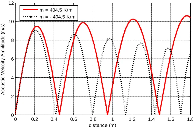
The distributions of the amplitudes of the acoustic pressure and velocity with different temperature gradients have been determined at a frequency of 700 Hz. The acoustic pressure and velocity amplitude versus axial distance in the impedance tube are shown in Figure 1 and Figure 2. The acoustic pressure amplitude is seen to be increasing along the length of the impedance tube while the wavelength reduces due to the decrease in temperature through the prescribed linear temperature gradient (T =1000+m.x) for m = – 404.5 K/m. When a positive value of temperature gradient is used, then longer wavelength is observed with a decrease in the acoustic pressure amplitude. The acoustic velocity amplitude in the impedance tube will decrease for negative values of the temperature gradient and increase for positive values of the temperature gradient as shown in Figure 2. The velocity and pressure anti-nodes and nodes are not evenly distributed along the axial distance of the impedance tube in the presence of a mean temperature gradient.
Figure 1: The acoustic pressure amplitude with axial distance in an impedance tube for different temperature profiles at 700 Hz for T0 = 1000 K.
0 0.2 0.4 0.6 0.8 1 1.2 1.4 1.6 1.8 0 500 1000 1500 2000 2500 3000 distance (m) A c ous ti c P res s ur e A m pl it ude ( P a)
Figure 2: The acoustic velocity amplitude with axial distance in an impedance tube for different temperature profiles at 700 Hz for T0 = 1000 K.
Sound is the mechanical energy propagating in a continuous, elastic medium by the compression
and rarefaction of particles [19]. Consider the movement of the air particles in a one-dimensional impedance tube. A sound source mounted at one end of the impedance tube is used to send sound waves. When sound source is turned on, the air particles next to it in the impedance tube will be vibrating forward and backward. As a result of the forward and backward motion, air particles cause high pressure areas known as compression where the particles have been squeezed together and low pressure areas known as rarefaction where the particles have been spread apart. As sound waves travelling in impedance tube the direction of the forward and backward motion of the air particles is parallel to the direction of wave propagation. Such waves are called longitudinal waves. When the waveform of sound produced by the source is sinusoidal then the resulting sound is a pure tone with a single frequency. The sound waves varying with time at any point in the tube will be sinusoidal. The amplitude of the sound waves will be zero at the transitional point where compressed air particles are starting to be decompressed or decompressed air particles are starting to be compressed. This means that the sinusoidal function has zero amplitude at zero time.
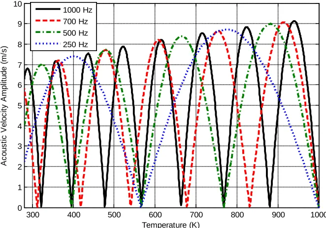
For a linear temperature gradient, the axial acoustic intensity in a sound wave remains constant along the length of an impedance tube. When the temperature gradient creates an increase in the acoustic pressure it will also create a consequent decrease in the axial velocity. Acoustic pressure and velocity amplitudes of one dimensional acoustic wave in impedance tube versus temperature have been calculated for frequencies of 1000 Hz, 700 Hz, 500 Hz and 250 Hz (see Figure 3 and Figure 4). When the frequency decreases, the number of pressure nodes and anti-nodes in the ducts decreases while the wavelength of the acoustic wave increases. Acoustic pressure amplitude existing in the duct decreases with increasing linear temperature. The acoustic velocity amplitude increases with increasing linear temperature. A shorter wavelength is observed at lower temperature and a larger wavelength is observed at higher temperature. Increasing the temperature cause an increase in the speed of sound on which the wavelength depends. This clearly can be seen from the Figure 3 and Figure 4. Acoustic pressure amplitudes and velocity
0 0.2 0.4 0.6 0.8 1 1.2 1.4 1.6 1.8 0
2 4 6 8 10 12
distance (m)
A
c
ous
ti
c
V
el
oc
it
y
A
m
pl
it
ude (
m
/s
)
amplitudes are zero at some temperatures where air particles are starting to be squeezed together from decompression or to be spread apart from compression because the time is zero at that temperature.
Figure 3: Acoustic pressure amplitude versus temperature at 1000 Hz, 700 Hz, 500 Hz and 250 Hz.
Figure 4: Acoustic velocity amplitude versus temperature at 1000 Hz, 700 Hz, 500 Hz and 250 Hz.
300 400 500 600 700 800 900 1000
0 500 1000 1500 2000 2500 3000
Temperature (K)
A
cous
tic
P
res
sur
e A
m
pl
itude (
P
a)
1000 Hz 700 Hz 500 Hz 250 Hz
300 400 500 600 700 800 900 1000
0 1 2 3 4 5 6 7 8 9 10
Temperature (K)
A
c
ous
ti
c
V
el
oc
it
y
A
m
pl
it
ude (
m
/s
)
Acoustic pressure amplitude for different temperature gradient has been investigated as a function of time at a position x = 20 cm along the impedance tube for a frequency of 1000 Hz and the results have been presented in Figure 5. Increasing the temperature gradient is shifting the wave form slightly to the left while the amplitude of the acoustic wave is decreasing. This is clearly due to the decreases in the pressure caused by increasing temperature in the tube. At a given frequency increasing the temperature in tube will cause an increase in speed of sound. Therefore the wavelength of the sound waves will increase too. The form of the acoustic waves has not been changed by varying temperature gradient.
Figure 5: Predicted acoustic pressure amplitude for different temperature gradients as a function of time at x = 20 cm from the inlet of tube for 1000 Hz.
3. CFD (Computational Fluid Dynamic) simulation of an impedance tube with mean temperature gradient
The Navier-Stokes simulations were obtained using ANSYS Fluent V13 [20]. A circular cross section impedance tube, of length 180 cm and diameter 7.5 cm was modelled as a 2D-axisymetric system with a regular mesh of 1800 x 120 cells in the axial and radial directions respectively. Solutions were obtained using the segregated pressure based solver with second order accurate discretisation in space and time. The effects of turbulence were assumed to be negligible in the absence of mean flow. A full Navier-Stokes simulation was obtained, retaining viscous terms and wall shear.
A linear temperature profile was defined as the thermal boundary condition along the outer wall of the impedance tube. An initial steady state solution was obtained to ensure a uniform varying temperature gradient through the gaseous medium, prior to imposing the acoustic pressure signal. Air in impedance tube is modelled as an ideal gas and its thermo-physical properties are given as specific heat = 1006.43 J/(kg K), thermal conductivity = 0.02424 W/(m K), and viscosity = 1.7894 x 10⁻⁵ kg/(m s). The wall of impedance tube is modelled as aluminium and its
thermo-1 2 3 4 5 6
x 10-3
-6 -4 -2 0 2 4 6
Time (s)
A
c
ous
ti
c
P
res
s
ur
e A
m
pl
it
ude (
P
a)
physical properties are given as density = 2719 kg/m3, specific heat = 871 J/(kg K), and thermal conductivity = 202.4 W/(m K). The end of impedance tube is a stationary wall which has zero absorption coefficients. Total reflection occurs at the end of impedance tube.
The acoustic pressure (gauge total pressure) at the inlet of the impedance tube was defined as a sinusoidal variation with initial amplitude, Ao, of 5 Pa.
) . 2 sin( )
(t P0 A0 f t
P = + π (7)
where P0 is the atmospheric pressure which is 101325 Pa, A0 is the sound pressure amplitude, f
is the frequency and t is the time.
A time accurate solution was obtained with a time step equal to 0.01 milliseconds. The resultant spatial and temporal resolution was demonstrated to accurately resolve the range of acoustic wavelengths and frequencies under consideration, with a spatial resolution of 340 cells for a wavelength at a frequency of 1000 Hz and a corresponding temporal resolution of 100 time steps per period. Time step size used for run calculation is 1x10⁻⁵ with 800 time steps. Maximum iteration per time step is 20. Profile update interval and reporting interval is 1. Total computational time is 8 milliseconds. The convergence history of acoustic-pressure for 8x10⁻³ s has been plotted for 4200 iterations.
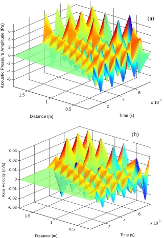
Figure 6: CFD simulation of acoustic-pressure as a function of axial length of the tube Numerical simulations of acoustic wave propagation varying by time and along the axial length of the tube were obtained for a range of frequencies and temperature gradient. Surface plots of acoustic pressure amplitude and axial velocity varying as a function of time and distance obtained at 1000 Hz and 700 Hz are presented in three-dimensions as shown in Figure 7, and Figure 8, respectively. The number of peaks observed as a function of time decreases when acoustic waves travel along the tube. Wavelength of acoustic waves is varying because of the changes in the linear temperature. Acoustic wave observed at the end of the impedance tube (x = 180 cm) obviously are combination of incident wave and reflected wave which formed a constructive interference and increased the amplitude of the acoustic wave. It can clearly be seen from the Figures 7 – 8 that incident waves and reflected waves are causing destructive and constructive standing waves. Acoustic waves in the impedance tube are longitudinal waves. Hot air particles vibrate parallel to the axial length of the impedance tube. The acoustic pressure amplitude of the vibration varies from a maximum pressure at the anti-nodes to pressure minima (zero) at the nodes. The vibration of the hot air particles disturbs the molecules at the pressure maxima, and causes them to shift and gather near the positions of the pressure minima. The hot air molecules on either side of pressure minima vibrate in antiphase while hot air molecules in the region between two close nodes vibrate in phases. Pressure amplitude peaks observed at 1000 Hz are more than peaks observed at 700 Hz. This is because of the wavelength at 1000 Hz is smaller than the wavelength at 700 Hz.
0 0.2 0.4 0.6 0.8 1 1.2 1.4 1.6 1.8
-5 -4 -3 -2 -1 0 1 2 3 4 5
Distance (m)
A
c
ous
ti
c
P
res
s
ur
e A
m
pl
it
ude (
P
Figure 7: (a) Surface plot of acoustic pressure amplitude and (b) surface plot of axial velocity amplitude versus time and distance at 1000 Hz.
2
4
6
x 10-3 0.5
1 1.5
-6 -4 -2 0 2 4 6
Time (s) Distance (m)
A
c
ous
ti
c
P
res
s
ur
e A
m
pl
it
ude (
P
a)
2
4
6
x 10-3 0.5
1 1.5
-0.02 -0.01 0 0.01 0.02
Time (s) Distance (m)
A
x
ia
l V
e
lo
c
it
y
(
m
/s
)
(a)
Figure 8: (a) Surface plot of acoustic pressure amplitude and (b) surface plot of axial velocity versus time and distance at 700 Hz.
Acoustic pressure amplitudes of acoustic waves in the impedance tube varying with time have been obtained at different position (x = 20 cm, x = 40 cm, x = 60 cm, x = 80 cm, x = 100 cm, x = 120 cm, x = 140 cm, x = 160 cm and x = 180 cm) in the tube for 700 Hz and 1000 Hz. The results are presented in Figure 9 and Figure 10. Constructive and destructive interferences between forward going waves and backward going waves can clearly be observed at some positions for 700 Hz and 1000 Hz. It is obvious that there is destructive interference between forward and backward going waves at the position of x = 160 cm for 700 Hz.
2 4
6
x 10-3
0.5 1
1.5 -6 -4 -2 0 2 4 6
Time (s) Distance (m)
A
c
ous
ti
c
P
res
s
ur
e A
m
pl
it
ude (
P
a)
2 4
6
x 10-3 0.5
1 1.5
-0.03 -0.02 -0.01 0 0.01 0.02 0.03
Time (s) Distance (m)
A
x
ia
l V
e
lo
c
it
y
(
m
/s
)
(a)
Figure 9: CFD data of acoustic pressure amplitudes versus time at the different position in the impedance tube with temperature gradient for 700 Hz.
Figure 10: CFD data of acoustic pressure amplitudes versus time at the different position in the impedance tube with temperature gradient for 1000 Hz.
0 1 2 3 4 5 6 7 8
x 10-3 -10
-8 -6 -4 -2 0 2 4 6 8 10
Time (s)
A
c
ous
ti
c
P
res
s
ur
e A
m
pl
it
ude (
P
a)
X = 180 cm X = 160 cm X = 140 cm X = 120 cm X = 100 cm X = 80 cm X = 60 cm X = 40 cm X = 20 cm
0 1 2 3 4 5 6 7 8
x 10-3
-8 -6 -4 -2 0 2 4 6 8
Time (s)
A
c
ous
ti
c
P
res
s
ur
e A
m
pl
it
ude (
P
a)
4. Comparison of between numerical simulation and analytical model
Data obtained from the numerical simulations at 20 cm and 180 cm form the inlet of the tube for 1000 Hz and 700 Hz are compared with the analytical model for one-dimensional oscillations in an impedance tube with an axial temperature gradient in the absence of mean flow. Acoustic pressure amplitudes versus time are presented in Figure 11 and Figure 12. The hot air molecules in the tube resonate with the frequency of the acoustic waves. This causes the peaks of sound intensity in the tube. It can be seen that hot air particles form into equally spaced peaks at the resonate frequencies. The agreement between numerical predictions and analytical model is shown to be very good.
Figure 11: Predictions compared with CFD data (a) at 20 cm and (b) at 180 cm from inlet for 1000 Hz.
Figure 12: Predictions compared with CFD data (a) at 20 cm and (b) at 180 cm from inlet for 800 Hz.
5. Conclusion and Further work
Numerical simulations of acoustic wave propagation through a temperature gradient in an impedance tube have been investigated. The results have been compared with the analytical model developed by Sujith et al. [2] for one-dimensional oscillations with an axial temperature gradient in the absence of mean flow. Surface and mesh plots of acoustic pressure and axial
1 2 3 4 5 6
x 10-3 -5 -4 -3 -2 -1 0 1 2 3 4 5 Time (s) A c ous ti c P res s ur e A m pl it ude ( P a) Prediction CFD
4 4.5 5 5.5 6 6.5 7 7.5 8
x 10-3 -8 -6 -4 -2 0 2 4 6 8 Time (s) A c ous ti c P res s ur e A m pl it ude ( P a) Prediction CFD
1 1.5 2 2.5 3 3.5 4 4.5 5 5.5 6
x 10-3
-6 -4 -2 0 2 4 6 Time (s) A c ous ti c P res s ur e A m pl it ude ( P a) Prediction CFD
4 4.5 5 5.5 6 6.5 7 7.5 8
x 10-3
-8 -6 -4 -2 0 2 4 6 8 Time (s) A c ous ti c P res s ur e A m pl it ude ( P a) Prediction CFD
a b
a
velocity amplitudes have been presented in 3-D against axial length of the tube and time. The agreement between numerical simulation and the analytical model is shown to be excellent and represents a baseline validation of the numerical methodology for the simulation of impedance tubes in the presence of temperature gradients.
Computational fluid dynamics results should be used to design an impedance tube for high temperature applications (e.g. gas turbine combustors), particularly with respect to location of microphones, by positioning them at the cool end of impedance tube but relating their measurements to what is actually happening at the hot end.
6. References
[1] A. Cummings, Ducts with axial temperature Gradients: an approximate solution for sound transmission and generation. Journal of Sound and Vibration 51 (1977) 55-67.
[2] R. I. Sujith, G. A. Waldherr, B. T. Zinn, An exact solution for one-dimensional acoustic fields in ducts with an axial temperature gradient. Journal of Sound and Vibration 184 (1995) 389-402.
[3] B. Karthik, B. M. Kumar, R. I. Sujith, Exact solutions to one-dimensional acoustic fields with temperature gradient and mean flow. J. Acoust. Soc. Am. 108 (2000) 38-43.
[4] R. I. Sujith, Exact solutions for modelling sound propagation through a combustion zone. J. Acoust. Soc. Am. 110 (2001), 1839 - 1844.
[5] K. S. Peat, The transfer matrix of a uniform duct with a linear temperature gradient. Journal of Sound and Vibration 123 (1988) 43-53.
[6] M. L. Munjal, M. G. Prasad, Plane-wave propagation in an uniform pipe in the presence of a mean flow and a temperature gradient. J. Acoust. Soc. Am. 80 (1986) 1501-1506.
[7] A. Kapur, A. Cummings, P. Mungur, Sound propagation in a combustion can with axial temperature and density gradients. Journal of Sound and Vibration 25 (1972) 129-138.
[8] H. Aygün, K. Attenborough, The insertion loss of perforated porous plates in a duct with and without mean air flow. Applied Acoustics 69 (2008) 506-513.
[9] H. Aygün, K. Attenborough, Sound absorption by clamped porous elastic plates. J. Acoust. Soc. Am. 124 (2008) 1-7.
[10] J. M. Middelberg, T. J. Barber, S. S. Leong, K. P. Byrne, and E. Leonardi, Computational Fluid Dynamics analysis of the acoustics performance of various simple expansion chamber mufflers. Proceedings of Acoustics. November 2004, Gold Coast, Australia.
[11] R. Kaess, W. Polifke, T. poinsot, N. Noiray, D. Durox, and T. Schuller, CFD-based mapping of the thermo-acoustic stability of a laminar premix burner. Center for Turbulenxe Research, Proceedings of the Summer Program 2008, 289-302.
[13] T. Lieuwen, & V. Yang, Combustion Instabilities in Gas Turbine Engines: Operational Experience, Fundamental Mechanisms, and Modelling. Progress in Astronautics and Aeronautics (2006). ISBN 156347669X. AIAA.
[14] C. Richter, Linear impedance modeling in the time domain with flow. Ph.D. Thesis, 2009, Technische Universitat Berlin, Germany.
[15] S. Dykas, W. Wroblewski, S. Rulik, and T. Chmielniak, Numerical method for modelling of acoustic waves propagation. Archives of Acoustics 35 (1), 2010, 35-48.
[16] L. Zhao, W. Qiao and L. Ji, Computational Fluid Dynamics simulation of sound propagation through a blade row. J. Acoust. Soc. Am. 132 (2012), 2210.
[17] J. Liu, Simulation of whistle noise using computational fluid dynamics and acoustic finite element simultion. MSc Thesis,University of Kentucky UKnowledge, 2012.
[18] E. Solberg, A wave propagation solver for Computational Aero-Acoustics. MSc Thesis, 2012. Chalmers University of Technology, Sweden.
[19] J. T. Bushberg, “The essential physics of medical imaging”, Williams & Wilkins, USA, 1994.