Orthogonality-Promoting Dictionary Learning via Bayesian Inference

The Thirty-Third AAAI Conference on Artificial Intelligence (AAAI-19)

Orthogonality-Promoting Dictionary Learning via Bayesian Inference

Lei Luo,

Jie Xu,

Cheng Deng,

Heng Huang

2_{School of Electronic Engineering, Xidian University, Xian, Shanxi, China,}3_{JDDGlobal.com}

[email protected], [email protected], [email protected], [email protected]

Abstract

Dictionary Learning (DL) plays a crucial role in numerous machine learning tasks. It targets at finding the dictionary over which the training set admits a maximally sparse rep-resentation. Most existing DL algorithms are based on solv-ing an optimization problem, where the noise variance and sparsity level should be known as the prior knowledge. How-ever, in practice applications, it is difficult to obtain these knowledge. Thus, non-parametric Bayesian DL has recently received much attention of researchers due to its adaptabil-ity and effectiveness. Although many hierarchical priors have been used to promote the sparsity of the representation in non-parametric Bayesian DL, the problem of redundancy for the dictionary is still overlooked, which greatly decreases the performance of sparse coding. To address this problem, this paper presents a novel robust dictionary learning frame-work via Bayesian inference. In particular, we employ the orthogonality-promoting regularization to mitigate correla-tions among dictionary atoms. Such a regularization, encour-aging the dictionary atoms to be close to being orthogonal, can alleviate overfitting to training data and improve the dis-crimination of the model. Moreover, we impose Scale mix-ture of the Vector variate Gaussian (SMVG) distribution on the noise to capture its structure. A Regularized Expecta-tion MaximizaExpecta-tion Algorithm is developed to estimate the posterior distribution of the representation and dictionary with orthogonality-promoting regularization. Numerical re-sults show that our method can learn the dictionary with an accuracy better than existing methods, especially when the number of training signals is limited.

Introduction

In the last decades, sparse coding, inspired by the sparsity mechanism of human vision system (Olshausen and Field 1996), has become a significant technique in computer vi-sion and machine learning with many real-world applica-tions such as image classification (Wright et al. 2009), visual tracking (Mei and Ling 2011) and cluster analysis (Elham-ifar and Vidal 2009). It models signals as linear combina-tions of a small number of atoms chosen from a large dic-tionary by solving anl0minimization problem. In addition

∗

Corresponding Author. L. Luo, H. Huang were partially sup-ported by U.S. NSF IIS 1836945, IIS 1836938, DBI 1836866, IIS 1845666, IIS 1852606, IIS 1838627, IIS 1837956.

Copyright c2019, Association for the Advancement of Artificial Intelligence (www.aaai.org). All rights reserved.

to solid theoretical studies (Candes and Tao 2005), numer-ous linear models following this line of sparse coding have recently emerged as powerful tools to cope with a variety of estimation tasks,e.g., Collaborative Representation Clas-sifier (CRC) (Zhang, Yang, and Feng 2011), Robust Sparse Coding (RSC) (Yang et al. 2011b), Nuclear norm based Ma-trix Regression (NMR) (Yang et al. 2017a), capped norm based robust dictionary learning (Jiang, Nie, and Huang 2015), and group sparsity based model (Nie et al. 2010; Yuan, Liu, and Ye 2011).

The dictionary plays an important role in these sparse rep-resentation based models. A desired dictionary learned from data often outperforms a set of predefined bases (Guo et al. 2016). As a result, dictionary learning (DL) has received a growing interest and a large number of DL algorithms have been proposed in recent years. K-SVD (Aharon, Elad, and Bruckstein 2006), as a classic DL algorithm, alternates be-tween sparse coding of the examples based on the current dictionary and a process of updating the dictionary atoms to better fit the data. However, K-SVD focuses on only the representational power of the dictionary (or the efficiency of sparse coding under the dictionary) without considering its capability for discrimination. To overcome this limitation, (Zhang and Li 2010) proposed a discriminative K-SVD al-gorithm to learn an over-complete dictionary from a set of labeled training face images. Different from (Zhang and Li 2010), (Yang et al. 2011a) employed the Fisher discrimi-nation criterion to learn a structured dictionary (FDDL for short). However, FDDL is not able to effectively represent the non-linear changes introduced by the pose variation. Thus (Shekhar et al. 2013) presented a robust supervised method for learning a single dictionary to optimally repre-sent both source and target data.

discriminative as possible, which may lead to sub-optimal classification performance. To alleviate this shortcoming, (You et al. 2018) considered a weak-supervision setting for analysis dictionary learning that is suitable for classification. priors.

The performance of the methods mentioned above is highly dependent on some prior knowledge such as noise variance and sparsity level (Chen et al. 2013) for choosing a proper regularizer. In practice, nevertheless, these prior in-formation are usually complex and unavailable. To mitigate this limitation, nonparametric Bayesian dictionary learn-ing algorithms (Zhou et al. 2009; 2012) are recently de-veloped. They cast dictionary learning as a factor-analysis problem, with the factor loading corresponding to the dic-tionary elements (atoms). Then, the model parameters are learned by utilizing nonparametric Bayesian techniques like the beta process (BP) (Paisley and Carin 2009), and the In-dian buffet process (IBP) (Ghahramani and Griffiths 2006), which circumvents arduous parameter adjustment task and explains DL models from the statistical perspective. To en-hance the discrimination of dictionary, (Akhtar, Shafait, and Mian 2016) adaptively built the association between the dic-tionary atoms with the class labels such that this associa-tion signifies the probability of selecassocia-tion of the dicassocia-tionary atoms in the expansion of classs-pecific data. Taking the un-certainty of the estimates in the inference process into ac-count, (Serra et al. 2017) presented a novel Bayesian ap-proach for thel1sparse dictionary learning problem based

on K-SVD. To promote the sparsity of the representation, (Yang et al. 2017b) leveraged a Gaussian-inverse Gamma hierarchical prior in modeling.

Although many supervised techniques (Akhtar, Mian, and Porikli 2017) can be integrated into Bayesian DL algo-rithms, they tried to improve the representation performance of sparse coding by constructing overcomplete dictionaries. This is obviously insufficient since such a strategy often re-sults in high computation cost and ambiguity in correspond-ing representations. Meanwhile, in many practical applica-tions, we may not learn a satisfactory dictionary due to the limited training samples. Thus, how to eliminate the redun-dancy among the dictionary atoms to improve the represen-tational power of sparse coding becomes an urgent problem to be solved.

Our Contributions. In this paper, we propose a novel Bayesian dictionary learning method. It uses the Orthogonality-Promoting regularization,i.e., BMD regular-izer (Xie et al. 2018), to mitigate correlations among the dictionary atoms. This regularizer encourages the dictionary atoms to be close to being orthogonal, which not only can alleviate overfitting to training data, but also improve the discrimination of the model. To facilitate the design of algorithm, we approximate the BMD regularizers with convex functions. Based on the basic framework of DL, we perform a Regularized Expectation Maximization of model parameters with the approximated BMD regularizer on the desired prior distribution. We model dictionaries, representation coefficients and noise under the Hierarchical formulation. Specially, we consider the relationship among elements of each noise vector using the Scale Mixture of

the Vector variate Gaussian (SMVG) distribution, which is a long-tail distribution and often is applied to robust modeling. This paper makes three main contributions:

• Based on the Hierarchical formulation, a novel non-parametric Bayesian dictionary learning model is intro-duced. It uses Orthogonality-Promoting regularization to eliminate the redundancy among the dictionary atoms, lead-ing to the stronger representation for sparse codlead-ing.

•To effectively estimate model parameters, a Regularized Expectation Maximization Algorithm is provided, which considers the structural information of the noise.

• Our experiments on four benchmark databases (AR, Extended Yale B, UCF sports action and Caltech-101 databases) show the superior performance of our method in classification tasks.

Preliminaries and Background

Notations

The bold capital and bold lowercase symbols are used to rep-resent matrices and vectors, respectively. The transpose of the matrixMis defined asMT. tr(M)and|M|(or det(M)) denote the trace and determinant of a square matrix M, respectively. exp(·) denotes the exponential function and etr(·) = exp(tr(·)).RandRl×m_{is the set of all real} num-ber and the set of all reall×m-dimensional matrices, re-spectively. For a matrix M, its i-th row is denoted by mi andmij denotes the(i, j)-th entry ofM. If al×l matrix

Mis positive semi-define, we denoteM 0orM ∈ R+_l .

E(M) and Cov(M) denote the expectation and covariance of M, respectively. Ip represents a p×p identity matrix.

z∼Nl(0,∆p)denotes that thep-dimensional vectorz fol-lows Gaussian distribution with zero mean and variance ma-trix∆p.k z k1 andk z k2denote the l1 andl2 of vector z, respectively.k M kF defines the Frobenius norm of the matrix M, which is equal to the l2-norm of Vec(M),i.e.,

kMkF=kVec(M)k2.∇φ(·)denotes the gradient of

func-tionφ(·).

Dictionary Learning

LetA= [a1,a2,· · ·,an]be a given dictionary, where each atomai∈ Rd. Considering the classical sparse coding task, a signaly∈ Rd_{can be approximately represented by a} lin-ear combination of a few atoms from the dictionaryAas:

y≈Ax=x1a1+x2a2+· · ·+xnan, (1)

wherex = [x1, x2,· · ·, xn] ∈ Rn is a sparse coefficient

vector. To this end,x is characterized by anl0-norm, which

leads to thel0-norm minimization problem.

However, the minimization ofl0-norm is an NP hard

prob-lem. Donoho proved that “for most large under-determined systems of linear equations, the minimal l1-norm

near-solution approximates the sparsest near-near-solution” (Donoho 2006), therefore recent research usually formulates the sparse coding problem as the minimization ofl1-norm,i.e.,

the coding coefficient can be got by solving the following equation:

minxky−Axk2

Cases Squared Frobenius Norm (SFN) Von Neumann divergence (VND) Log-Determinant Divergence (LDD)

φ(X) kXk2

F tr(XlogX−X) −logdetX

Λφ(X,Y) kX−Yk2F tr(XlogX−XlogY−X+Y) tr(XY

−1_{)−logdet(XY}−1₎ Λφ,con(X,Y) kX−Yk2F +tr(X) tr((X+εY)log(X+εY)) −logdet(X+εY) + (log

1

ε)tr(X)

Table 1: Three different cases forφ(X), which induce three BMDs, whereε >0is a small scalar

whereα > 0 is a balance parameter. In (2), the first term is called as reconstruction error, and the second term is the sparsity penalty.

The choice of dictionaryAdominates the representation performance of coefficientsx. To obtain a better dictionary from the training set ofksamplesY = [y₁,y₂,· · ·,y_k] ∈

Rd×k, many dictionary learning (DL) algorithms have been proposed, the basic idea of which is to minimize the follow-ing empirical cost function over both a dictionaryAand a sparse coefficients matrixX = [x1,x2,· · ·,xk]∈ Rd×k:

minA,XkY−AXk2F +βkXk1

s.t., kaik22≤1, ∀ i= 1,2,· · ·, n,

(3)

whereβ >0is a balance parameter. The constraintkaik22≤ 1 targets at preventing dictionary Afrom being arbitrarily large because it would cause very small values of coeffi-cients matrix X. In (3), one seeks to match the dictionary

Ato the imagery of interest, while simultaneously encour-aging a sparse representationX.

Orthogonality-Promoting Regularization

Orthogonality-promoting regularization, preventing the re-dundancy among the learned variables, has been recently studied in some machine learning problems including la-tent variable modeling, multitask learning and metric learn-ing (Xie et al. 2018). Due to the easy convex relaxation and complete theoretical guarantee, we choose BMD regularizer as an orthogonality-promoting regularization in this paper.

Definition 1. Given a strictly convex, differentiable func-tionφ : Rl×m −→ R. For any two real symmetric matrix

X,Y∈Rl×l, a BMD is defined as:

Λφ(X,Y) =φ(X)−φ(Y)−tr((∇φ(Y))T(X−Y)). (4)

Different functions φ can induce different versions of BMD, which can been used to measure thecloseness be-tween two matrices. According to (Xie et al. 2018), we sum-marize three cases aboutφin Table 1. The second line of Ta-ble 1 shows three popularφfunctions, which generate three BMDs,i.e., Squared Frobenius Norm (SFN), Von Neumann divergence (VND) and Log-Determinant Divergence (LDD) as displayed in the third line of Table 1. The convex relax-ations for three different BMDs are described in the last line of Table 1.

Proposed Method

In this section, we first describe our Hierarchical model for dictionary learning, then provide a Regularized Stochastic Variational Inference (RSVI) to estimate model parameters.

Overview of the Proposed Framework

Most of the compressive sensing literature assumes “off-the-shelf” wavelet and DCT bases/dictionaries, but recent de-noising and inpainting research has demonstrated the signif-icant advantages of learning an often over-complete dictio-nary matched to the signals of interest. In previous section, we revisited the basic sparse dictionary learning model. For the convenience, we rewritten it as:

Y=AX+E, (5)

whereE= [e1,e2,· · ·,ek]is the representation error matrix. Our goal is to estimate the optimal dictionary A and representation coefficients matrixXaccording to the given prior information. From statistical viewpoint, model (3) as-sumes each xi follows independent identically distributed (i.i.d.) with Laplace distribution, while each error vector

ei is characterized using independent Gaussian distribu-tion. However, these simple priors cannot cope with those complex data from real-world (Luo et al. 2018). To ad-dress this issue, in the following, we develop a hierarchi-cal Bayesian model with orthogonality-promoting regular-ization for learning dictionaries.

Modeling error matrix E. In Bayesian modeling, we need introduce a prior distribution on error matrix E. The scale mixture of the Gaussian distribution (Luo et al. 2018) belongs to the category of the elliptically contoured distri-bution. Compared with Gaussian distribution, it has heavier tails, which is beneficial for robust modeling. Meanwhile, considering the correlation between elements of the practical noise matrixE, Scale mixture of the Vector variate Gaussian (SMVG) distribution is used to model it in the first layer. That is,

ei =U−

1/w

i Φ

−1/2

i zi, (6)

wherezi ∼ Nd(0,Id),i = 1,2,· · · , k andw > 0. Each

Φi is called precision matrix. Eachei is controlled by the nonnegative parameterUi which is similar to the weight of each group in group sparsity (Yuan, Liu, and Ye 2011).

Settingwas2, (6) is equivalent to

P(ei|Φi, Ui,xi) =

|UiΦi|

(2π)d/2exp

−1

2e

T

i(UiΦi)ei

. (7)

SinceE=Y−AX, (7) is rewritten as P(y_i|Φi, Ui,xi,A)

= |UiΦi| (2π)d/2exp

−1

2(yi− Axi)

T

(UiΦi)(yi− Axi)

.

(8)

Suppose different samples are independent of each other. Then, we have

P(Y|Φ,U,X,A) =

k Y

i

P(y_i|Φi, Ui,xi,A). (9)

HereΦ= [Φ1,Φ2,· · ·,Φk]andU= [U1, U2,· · ·, Uk].

In the second layer, we use Jeffrey’s prior to fit each scalar variableUiaccording to (Luo et al. 2018). Then,

P(U) =

k Y

i=1

P(Ui)∝

k Y

i=1 1

Ui. (10)

Gamma distribution (Luo et al. 2018) is one of the most widely used prior for the precision matrix Φi of the ran-dom effects since it provides a convenient conjugate prior for multivariate normal distribution. Thus, for each super pa-rameterΦi, we impose the matrix variate Gamma prior on it,i.e.,

P(Φi) =

Td(c)|Wi|−c

−1

|Φi|c−

1

2(d+1)_etr(−_WΦi),

(11)

whereTd(c) is a multivariate gamma function (Luo et al. 2018).

Modeling dictionary A. Similarly, to effectively model dictionaryA, we use the scale mixture of the Vector variate Gaussian distribution to fit it under Hierarchical formula-tion,i.e.,

ai=V −1/w

i Ψ

−1/2

i gi, (12)

wheregi∼Nd(0,Id),i= 1,2,· · ·, k, and eachai>0. Lettingw= 2, we have

P(ai|Ψi, Vi) =

|ViΨi|

(2π)d/2exp

−1

2a

T

i(ViΨi)ai

. (13)

Assuming that different atoms are independent of each other, we have

P(A|Ψ,V) =

k Y

i

P(ai|Ψi, Ui), (14)

whereΨ= [Ψ1,Ψ2,· · · ,Ψk]andV= [V1, V2,· · ·, Vk].

In the second layer, we impose Jeffrey??s prior on each scalar variableVi,i.e.,

P(V) =

k Y

i=1

P(Vi)∝

k Y

i=1 1

Vi. (15)

Meanwhile, matrix variate Gamma prior is chosen as the prior distribution of eachΦi,i.e.,

P(Ψi) =

Tn(c)|Wi| −c−1

|Ψi|c−

1

2(n+1)_etr(−_WΨ_i).

(16)

Modeling coefficients matrix X. In the first layer, ele-ments in the coefficient vectorxare assumed to be indepen-dent and follow the scale mixture of the univariate Gaussian distribution, which has been extensively used to exploit the sparsity ofxj(Luo et al. 2018). That being said,

xij = (γij)−1/2zij, (17)

wherezij ∼N(0,1),(γij)−1is the precision ofxij, andxij is thei-th element ofxj. This is equivalent to setting

P(xij) = r

γij

2πexp(−γij(xij)

2_{/2) =N(x}

ij|0,(γij)−1). (18) Let γj = [γj1, γj2,· · ·, γjn]T and γjdiag = diag(γ1j, γ2j,· · ·, γnj), then (18) can be re-expressed

as:

P(xj|γj) =

|γj|

(2π)n/2exp

−1 2x T jγ diag j xj

. (19)

Thus,

P(X|γ) = Πk_j=1P(xj|γj), (20) where γ = [γ1,γ2,· · · ,γk]. The second layer specifies Gamma distributions as hyper priors over each hyper param-etersγiin our method. Therefore,

P(γj) = Πkj=1P(γij) = Π

k

j=1Gamma(γij|a+ 1, b)

= Πk_j=1 b

a+1

Γ(a+ 1)γ

a

ijexp(−bγij).

(21)

Regularized Expectation Maximization (REM)

Algorithm

The EM algorithm (McLachlan and Krishnan 2007) is a gen-eral methodology for maximum likelihood (ML) or MAP estimation. The recent emphasis in the sparse or low-rank reconstruction literature on probabilistic models has led to the increased interest in EM. The EM algorithm starts from an initial guess and iteratively runs an expectation (E) step, which evaluates the posterior probabilities using currently estimated parameters, and a maximization (M) step, which re-estimates the parameters based on the probabilities cal-culated in theE step. The iterations will not stop until the convergence conditions are satisfied.

In our method, we consider dictionaryAand representa-tion coefficientsXas the hidden variable. Thus, forE-step, based on the current parameters, the Maximum-A Posteri-ori (MAP) estimate ofX, denoted asXˆ, can be achieved by solving the following problem:

ˆ

X=argmax_XP(X|A,Y,Φ,U,γ,Ψ,V)

=argmax_XP(Y|Φ,U,X,A)P(X|γ)P(A|Ψ,V). (22)

Similarly, the Maximum-A Posteriori (MAP) estimate of

A, denoted asAˆ, can be achieved by solving the following problem:

ˆ

A=argmax_AP(A|X,Y,Φ,U,γ,Ψ,V)

Let

LA=P(Y|Φ,U,X,A)P(X|γ)P(A|Ψ,V). (24)

To encourage the dictionary atoms to be close to being or-thogonal, we use BMD regularizers to constrain dictionary atoms. Then, (23) becomes:

ˆ

A=argmin_A−lnLA+ρΛφ,con(ATA,In)

. (25)

For Eq. (22), we can obtain a closed-form solution by computing its derivative. However, for Eq. (25), we only can iteratively calculate it. Here we adopt stochastic proximal subgradient method to optimize it,i.e.,

A(t)←prox_η(t)_R(A(t−1)−η(t)

· ∇(lnL_A(t−1)+ρΛφ,con(A(t−1) T

A(t−1),In)), (26)

where

prox_R(B) =argmin_A∈Rd×n{

1

2 kA−Bk 2

F +R(A)} (27) is a proximal mapping.

In the M-step, using the current posterior probabilities, parametersΘ={γ,Φ,U,Ψ,V}can be obtained by mini-mizing the following help function:

Q(Θ,Θold) +logP(Θ), (28)

whereΘold_{includes the values of parameters from the} pre-vious iteration andQ(Θ,Θold_{)can be defined as}

Q(Θ,Θold) =EX|Y,A,Θold[logP(X,A,Y|Θ)], (29) and

P(Θ) =P(γ)P(Φ)P(U)P(Ψ)P(V). (30)

Taking the stationary point of the objective function (28) with respect to each parameter, we can obtain their solutions. In fact, we can equivalently write the basic iterative proce-dure as follows:

X ←argmax_XP(X|A,Y,Φ,U,γ,Ψ,V); (31)

ˆ

A←argmin_A−lnLA+ρΛφ,con(ATA,In)

; (32)

γ←argmax_γ,Φ,U,Ψ,VP(γ,Φ,U,Ψ,V). (33)

Φ←argmax_γ,Φ,U,Ψ,VP(γ,Φ,U,Ψ,V). (34)

U←argmax_γ,Φ,U,Ψ,VP(γ,Φ,U,Ψ,V). (35)

Ψ←argmax_γ,Φ,U,Ψ,VP(γ,Φ,U,Ψ,V). (36)

V←argmax_γ,Φ,U,Ψ,VP(γ,Φ,U,Ψ,V). (37) The prior distribution for each parameter has been given in the previous section. As we know, the complexity of stan-dard EM algorithm for estimating model parameters is very high. To circumvent this shortcoming, we can use stochas-tic EM (SEM) algorithm (Dombry et al. 2017) to train our model. The basic idea of SEM algorithm is to randomly choose training sample and compute the corresponding so-lution in each step. But here, we omit the detailed iterative procedure.

Experiments

We evaluated the performance of the proposed approach on two face data sets: the AR (Martinez 1998) and the Extended YaleB (Lee and J. Ho 2005) for face recognition, a data set for action recognition: UCF sports action (Rodriguez, Ahmed, and Shah 2008) and a data set for object categories: Caltech-101 (Lazebnik, Schmid, and Ponce 2006). These data sets are commonly used in the related literature for eval-uation of matrix regression and dictionary learning models. Meanwhile, our method is compared with some representa-tive methods such as Sparse Representation based classifi-cation (SRC) (Wright et al. 2009), Collaborative Represen-tation based Classification (CRC) (Zhang, Yang, and Feng 2011), K-SVD (Aharon, Elad, and Bruckstein 2006), Fisher Discrimination Dictionary Learning (FDDL) (Yang et al. 2011a), Label Consistent K-SVD (LS-KSVD) (Jiang, Lin, and Davis 2013), Beta Process Construction (BPC) (Zhou et al. 2009) and Nonparametric Bayesian Correlated Group Regression (BCGR) (Luo et al. 2018). Specifically, SRC and CRC belong to the category of the matrix regression. BCGR is a nonparametric Bayesian matrix regression method. K-SVD, FDDL and LS-KSVD are classical dictionary learn-ing methods. BPC is the well-known Bayesian dictionary learning method, which considers beta process as a prior for learning a dictionary. According to the suggestion of (Luo et al. 2018), we seta, b, c= 10−4. To be fair, we adopt the sparse representation based classifier.

Databases

The AR face databasecontains over 4,000 color face im-ages of 126 people, including frontal views of faces with dif-ferent facial expressions, lighting conditions and occlusions. The pictures of most persons were taken in two sessions (separated by two weeks). Each section contains 13 color images and 120 individuals (65 men and 55 women) partic-ipated in both sessions. The images of these 120 individu-als were selected and used in our experiment. We projected

165×120cropped face images onto 540-dimensional vec-tors using a random projection matrix (Wright et al. 2009), thereby extracting Random-Face features.

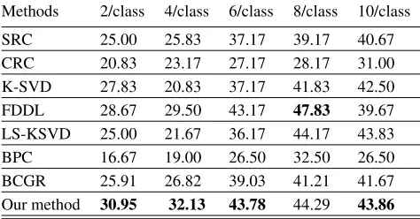
Methods 2/class 4/class 6/class 8/class 10/class

SRC 25.00 25.83 37.17 39.17 40.67 CRC 20.83 23.17 27.17 28.17 31.00 K-SVD 27.83 20.83 37.17 41.83 42.50 FDDL 28.67 29.50 43.17 47.83 39.67 LS-KSVD 25.00 21.67 36.17 44.17 43.83 BPC 16.67 19.00 26.50 32.50 26.50 BCGR 25.91 26.82 39.03 41.21 41.67 Our method 30.95 32.13 43.78 44.29 43.86

Table 2: Classification accuracy (%) for sunglasses disguise on the AR face Database

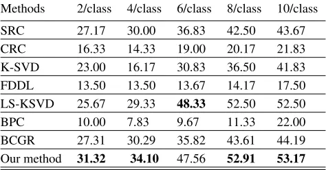
Methods 2/class 4/class 6/class 8/class 10/class

SRC 27.17 30.00 36.83 42.50 43.67 CRC 16.33 14.33 19.00 20.17 21.83 K-SVD 23.00 16.17 30.83 36.50 41.83 FDDL 13.50 13.50 13.67 14.17 17.50 LS-KSVD 25.67 29.33 48.33 52.50 52.50 BPC 10.00 7.83 9.67 11.33 22.00 BCGR 27.31 30.29 35.82 43.61 44.19 Our method 31.32 34.10 47.56 52.91 53.17

Table 3: Classification accuracy (%) for scarf disguise on the AR face Database

light source direction and the camera axis. The 64 images of a subject in a particular pose are acquired at camera frame rate of 30 frames/s, so there is only small change in head pose and facial expression for those 64 images. Here we create 504-dimensional random face features (Wright et al. 2009) from the192×168cropped face images.

Caltech-101 database contains 9, 144 image samples from 101 object categories and a class of background im-ages. The number of samples per class in this database vary between 31 and 800. For classification, we first cre-ated 4096- dimensional feature vectors of the images using the 16- layer deep convolutional neural networks for large scale visual recognition. These features were used to create the training and the testing data sets

UCF sports action databaseconsists of a set of actions collected from various sports which are typically featured on broadcast television channels such as the BBC and ESPN. The video sequences were obtained from a wide range of stock footage websites including BBC Motion gallery and GettyImages. The dataset includes a total of 150 sequences with the resolution of 720×480. The collection represents a natural pool of actions featured in a wide range of scenes and viewpoints. By releasing the data set we hope to en-courage further research into this class of action recognition in unconstrained environments. Since its introduction, the dataset has been used for numerous applications such as: action recognition, action localization, and saliency detec-tion. We used the action bank features (Sadanand and Corso 2012) for this database to train and test our approach.

Experiments on the AR face database

Two groups of experiments are designed on the AR face database. In the first experiment, we test the performance of our method under different number of training samples. As we know, AR face database contains 14 face images without real disguise for each person. We randomly choose 2, 4, 6, 8 or 10 face images from them as training samples. Then, three face images with sunglasses and three face images with scarf from session 1 are considered as test samples, respectively. Tables 2 and 3 report the classification accura-cies of SRC, CRC, K-SVD, FDDL, LS-KSVD, BPC, BCGR and our method for the two cases under different number of

training samples. The advantage of our method is more ob-vious with the decreasing of number of training samples. Es-pecially, when there are less than 6 training samples, at least 2.28% improvement is achieved by our methods compared to other method. Although both SRC and BCGR exclusively handle occlusion problem, they rely on overcomplete dic-tionary. Therefore, for small samples, our method perform better than these two methods.

We conduct the second experiment on session 1 from the AR face database. A random subset with three per subject is chosen to form the training set and the rest are taken as the testing set. The experiment is repeated over five random splits of the data set. The second line of Table 4 lists the average classification accuracies and standard deviations of all methods. It can be observed that the proposed method has a leading performance. It achieves an improvement of more than 2% as compared to the second best method: FDDL. The Bayesian dictionary learning method BPC seems to perform poorly at handling occlusions.

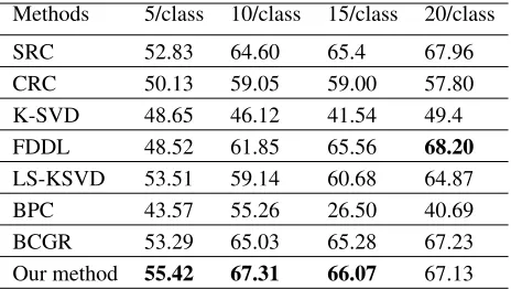
Experiments on the Extended Yale B database

Similar to the previous experiment, the first {5, 10, 15, 20} face images for each class from the Extended YaleB database are chosen as training set, the rest are taken as the testing set. The experimental results of each method are dis-played in Table 5. It can be found that our method gives bet-ter classification accuracy. With the decreasing of number of training samples, the advantage of our method is more clear as we expected. Meanwhile, FDDL shows a competi-tive performance for “20/class” (68.20%). In the second ex-periment, the Extended YaleB data is randomly split into two subsets with thirty-four persons each. One for training and the other for testing. We repeat the process five times to ob-tain the results over the five testing sets. The mean classifi-cation accuracy and standard deviations over the 5 training set for each algorithm are detailed in the third line of Ta-ble 4. It is easy to see that our method is superior to other methods. Meanwhile, SRC (97.85%) and BCGR (97.12%) outperform K-SVD (71.07%) and BPC (83.41%). The clas-sification accuracy of LS-KSVD is 97.53% which is higher than FDDL by 2.47%. On the Extended Yale B database, SRC, LS-KSVD and BCGR is robust to illumination. Their classification accuracies are: 97.85%, 71.07% and 97.12%.

Experiments on the UCF sports action database

Databases SRC CRC K-SVD LS-KSVD FDDL BPC BCGR Our method

AR 90.27±1.28 72.83±1.67 79.23±1.77 87.40±1.26 89.20±1.37 35.52±2.35 86.78±1.53 91.72±1.31 Extended Yale B 97.85±0.41 87.15±1.13 71.07±1.80 97.53±0.71 94.79±0.39 83.41±0.28 97.12±1.06 97.87±1.51

UCF sports 89.86±2.29 87.54±4.87 81.16±2.05 73.62±8.03 83.77±3.30 84.35±2.97 86.14±2.79 91.38±3.02

Caltech-101 97.35±0.17 88.28±0.33 80.64±2.81 97.83±0.23 91.35±0.10 89.26±0.60 92.18±0.56 97.91±0.82

Table 4: Classification accuracy (%) and standard deviations on the AR, Extended Yale B database, UCF sports action databases and Caltech-101 database.

Methods 5/class 10/class 15/class 20/class

SRC 52.83 64.60 65.4 67.96

CRC 50.13 59.05 59.00 57.80

K-SVD 48.65 46.12 41.54 49.4

FDDL 48.52 61.85 65.56 68.20

LS-KSVD 53.51 59.14 60.68 64.87

BPC 43.57 55.26 26.50 40.69

BCGR 53.29 65.03 65.28 67.23

Our method 55.42 67.31 66.07 67.13

Table 5: Classification accuracy (%) on the Extended Yale Database

Experiments on the Caltech-101 database

In this section, we implement an experiment on the Caltech-101 database for object recognition. For this data set, we directly use the 3000-dimensional Spatial Pyramid Features of the images provided by Jianget al.(Jiang, Lin, and Davis 2013). From these features, 15 random samples per class are used for training and the remaining samples for testing. The experimental results on this database are summarized in the last line of Table 4. It is seen that the performance of our method is similar to that of SRC and LS-KSVD. Especially, LS-KSVD performs better than K-SVD, which indicates the label information may be beneficial for classification task. BPC (84.35%), as a Bayesian dictionary learning method, has the higher accuracy as compared to K-SVD.

Conclusions

This paper proposed a non-parametric Bayesian approach for learning a desired dictionary. We hierarchically model each parameter and estimate them using a Regularized Ex-pectation Maximization Algorithm. To eliminate the redun-dancy of the dictionary atoms, we force a orthogonality-promoting regularization on the dictionary matrix, which improves the performance of sparse coding and the discrim-ination of the model. A series of experiments on four bench-mark databases demonstrate that the proposed model can ef-fectively cope with the practical classification problem, par-ticularly for the case where there is a limited number of training samples.

References

Aharon, M.; Elad, M.; and Bruckstein, A. 2006. rmk-svd: An algorithm for designing overcomplete dictionaries for sparse representation. IEEE Transactions on signal pro-cessing54(11):4311–4322.

Akhtar, N.; Mian, A. S.; and Porikli, F. 2017. Joint discrimi-native bayesian dictionary and classifier learning. InCVPR, 3919–3928.

Akhtar, N.; Shafait, F.; and Mian, A. 2016. Discrimina-tive bayesian dictionary learning for classification. IEEE transactions on pattern analysis and machine intelligence 38(12):2374–2388.

Candes, E. J., and Tao, T. 2005. Decoding by linear programming. IEEE transactions on information theory 51(12):4203–4215.

Chen, B.; Polatkan, G.; Sapiro, G.; Blei, D.; Dunson, D.; and Carin, L. 2013. Deep learning with hierarchical convolu-tional factor analysis.IEEE transactions on pattern analysis and machine intelligence35(8):1887–1901.

Dombry, C.; Genton, M. G.; Huser, R.; and Ribatet, M. 2017. Full likelihood inference for max-stable data. arXiv preprint arXiv:1703.08665.

Donoho, D. L. 2006. For most large underdetermined sys-tems of linear equations the minimal ??1-norm solution is also the sparsest solution.Communications on Pure and Ap-plied Mathematics: A Journal Issued by the Courant Insti-tute of Mathematical Sciences59(6):797–829.

Elhamifar, E., and Vidal, R. 2009. Sparse subspace clus-tering. InComputer Vision and Pattern Recognition, 2009. CVPR 2009. IEEE Conference on, 2790–2797. IEEE.

Ghahramani, Z., and Griffiths, T. L. 2006. Infinite latent feature models and the indian buffet process. InAdvances in neural information processing systems, 475–482.

Guo, J.; Guo, Y.; Kong, X.; Zhang, M.; and He, R. 2016. Discriminative analysis dictionary learning. InAAAI, 1617– 1623.

Jiang, Z.; Lin, Z.; and Davis, L. S. 2013. Label consistent k-svd: Learning a discriminative dictionary for recognition. IEEE transactions on pattern analysis and machine intelli-gence35(11):2651–2664.

Lazebnik, S.; Schmid, C.; and Ponce, J. 2006. Beyond bags of features: Spatial pyramid matching for recognizing natu-ral scene categories. Innull, 2169–2178. IEEE.

Lee, K., and J. Ho, D. K. 2005. Acquiring linear subspaces for face recognition under variable lighting. IEEE Trans. on PAMI27(5):684–698.

Luo, L.; Yang, J.; Zhang, B.; Jiang, J.; and Huang, H. 2018. Nonparametric bayesian correlated group regression with applications to image classification. IEEE Transactions on Neural Networks and Learning Systems(99):1–15.

Martinez, A. M. 1998. The ar face database.CVC Technical Report24.

McLachlan, G., and Krishnan, T. 2007. The EM algorithm and extensions, volume 382. John Wiley & Sons.

Mei, X., and Ling, H. 2011. Robust visual tracking and vehicle classification via sparse representation. IEEE transactions on pattern analysis and machine intelligence 33(11):2259–2272.

Nie, F.; Huang, H.; Cai, X.; and Ding, C. H. 2010. Efficient and robust feature selection via joint ?2, 1-norms minimiza-tion. InAdvances in neural information processing systems, 1813–1821.

Olshausen, B. A., and Field, D. J. 1996. Emergence of simple-cell receptive field properties by learning a sparse code for natural images. Nature381(6583):607.

Paisley, J., and Carin, L. 2009. Nonparametric factor analy-sis with beta process priors. InProceedings of the 26th An-nual International Conference on Machine Learning, 777– 784. ACM.

Rodriguez, M. D.; Ahmed, J.; and Shah, M. 2008. Ac-tion mach a spatio-temporal maximum average correlaAc-tion height filter for action recognition. InComputer Vision and Pattern Recognition, 2008. CVPR 2008. IEEE Conference on, 1–8. IEEE.

Sadanand, S., and Corso, J. J. 2012. Action bank: A high-level representation of activity in video. InComputer Vi-sion and Pattern Recognition (CVPR), 2012 IEEE Confer-ence on, 1234–1241. IEEE.

Serra, J. G.; Testa, M.; Molina, R.; and Katsaggelos, A. K. 2017. Bayesian k-svd using fast variational inference.IEEE Transactions on Image Processing26(7):3344–3359. Shekhar, S.; Patel, V. M.; Nguyen, H. V.; and Chellappa, R. 2013. Generalized domain-adaptive dictionaries. In Pro-ceedings of the IEEE Conference on Computer Vision and Pattern Recognition, 361–368.

Wang, H.; Nie, F.; Cai, W.; and Huang, H. 2013. Semi-supervised robust dictionary learning via efficient l-norms minimization. In Proceedings of the IEEE International Conference on Computer Vision, 1145–1152.

Wright, J.; Yang, A. Y.; Ganesh, A.; Sastry, S. S.; and Ma, Y. 2009. Robust face recognition via sparse representation. IEEE transactions on pattern analysis and machine intelli-gence31(2):210–227.

Xie, P.; Wu, W.; Zhu, Y.; and Xing, E. P. 2018. Orthogonality-promoting distance metric learning:

Con-vex relaxation and theoretical analysis. arXiv preprint arXiv:1802.06014.

Yang, M., and Chen, L. 2017. Discriminative semi-supervised dictionary learning with entropy regularization for pattern classification. InAAAI, 1626–1632.

Yang, M.; Zhang, L.; Feng, X.; and Zhang, D. 2011a. Fisher discrimination dictionary learning for sparse representation. InComputer Vision (ICCV), 2011 IEEE International Con-ference on, 543–550. IEEE.

Yang, M.; Zhang, L.; Yang, J.; and Zhang, D. 2011b. Ro-bust sparse coding for face recognition. In Computer Vi-sion and Pattern Recognition (CVPR), 2011 IEEE Confer-ence on, 625–632. IEEE.

Yang, J.; Luo, L.; Qian, J.; Tai, Y.; Zhang, F.; and Xu, Y. 2017a. Nuclear norm based matrix regression with appli-cations to face recognition with occlusion and illumination changes. IEEE transactions on pattern analysis and ma-chine intelligence39(1):156–171.

Yang, L.; Fang, J.; Cheng, H.; and Li, H. 2017b. Sparse bayesian dictionary learning with a gaussian hierarchical model. Signal Processing130:93–104.

You, Z.; Raich, R.; Fern, X. Z.; and Kim, J. 2018. Weakly supervised dictionary learning.IEEE Transactions on Signal Processing66(10):2527–2541.

Yuan, L.; Liu, J.; and Ye, J. 2011. Efficient methods for overlapping group lasso. InAdvances in Neural Information Processing Systems, 352–360.

Zhang, Q., and Li, B. 2010. Discriminative k-svd for dic-tionary learning in face recognition. In Computer Vision and Pattern Recognition (CVPR), 2010 IEEE Conference on, 2691–2698. IEEE.

Zhang, L.; Yang, M.; and Feng, X. 2011. Sparse repre-sentation or collaborative reprerepre-sentation: Which helps face recognition? InComputer vision (ICCV), 2011 IEEE inter-national conference on, 471–478. IEEE.

Zhou, M.; Chen, H.; Ren, L.; Sapiro, G.; Carin, L.; and Pais-ley, J. W. 2009. Non-parametric bayesian dictionary learn-ing for sparse image representations. InAdvances in neural information processing systems, 2295–2303.