Online Passive-Aggressive Algorithms
Koby Crammer∗ [email protected]
Ofer Dekel [email protected]
Joseph Keshet [email protected]
Shai Shalev-Shwartz [email protected]
Yoram Singer† [email protected]
School of Computer Science and Engineering The Hebrew University
Jerusalem, 91904, Israel
Editor: Manfred K. Warmuth
Abstract
We present a family of margin based online learning algorithms for various prediction tasks. In particular we derive and analyze algorithms for binary and multiclass categorization, regression, uniclass prediction and sequence prediction. The update steps of our different algorithms are all based on analytical solutions to simple constrained optimization problems. This unified view al-lows us to prove worst-case loss bounds for the different algorithms and for the various decision problems based on a single lemma. Our bounds on the cumulative loss of the algorithms are relative to the smallest loss that can be attained by any fixed hypothesis, and as such are applicable to both realizable and unrealizable settings. We demonstrate some of the merits of the proposed algorithms in a series of experiments with synthetic and real data sets.
1. Introduction
In this paper we describe and analyze several online learning tasks through the same algorithmic prism. We first introduce a simple online algorithm which we call Passive-Aggressive (PA) for on-line binary classification (see also (Herbster, 2001)). We then propose two alternative modifications to the PA algorithm which improve the algorithm’s ability to cope with noise. We provide a unified analysis for the three variants. Building on this unified view, we show how to generalize the binary setting to various learning tasks, ranging from regression to sequence prediction.
The setting we focus on is that of online learning. In the online setting, a learning algorithm ob-serves instances in a sequential manner. After each observation, the algorithm predicts an outcome. This outcome can be as simple as a yes/no (+/−) decision, as in the case of binary classification problems, and as complex as a string over a large alphabet. Once the algorithm has made a predic-tion, it receives feedback indicating the correct outcome. Then, the online algorithm may modify its prediction mechanism, presumably improving the chances of making an accurate prediction on subsequent rounds. Online algorithms are typically simple to implement and their analysis often provides tight bounds on their performance (see for instance Kivinen and Warmuth (1997)).
∗. Current affiliation: Department of Computer and Information Science, University of Pennsylvania, 3330 Walnut Street, Philadelphia, PA 19104, USA.
Our learning algorithms use hypotheses from the set of linear predictors. While this class may seem restrictive, the pioneering work of Vapnik (1998) and colleagues demonstrates that by us-ing Mercer kernels one can employ highly non-linear predictors and still entertain all the formal properties and simplicity of linear predictors. For concreteness, our presentation and analysis are confined to the linear case which is often referred to as the primal version (Vapnik, 1998; Cristianini and Shawe-Taylor, 2000; Sch¨olkopf and Smola, 2002). As in other constructions of linear kernel machines, our paradigm also builds on the notion of margin.
Binary classification is the first setting we discuss in the paper. In this setting each instance is represented by a vector and the prediction mechanism is based on a hyperplane which divides the instance space into two half-spaces. The margin of an example is proportional to the distance between the instance and the hyperplane. The PA algorithm utilizes the margin to modify the current classifier. The update of the classifier is performed by solving a constrained optimization problem: we would like the new classifier to remain as close as possible to the current one while achieving at least a unit margin on the most recent example. Forcing a unit margin might turn out to be too aggressive in the presence of noise. Therefore, we also describe two versions of our algorithm which cast a tradeoff between the desired margin and the proximity to the current classifier.
The above formalism is motivated by the work of Warmuth and colleagues for deriving online algorithms (see for instance (Kivinen and Warmuth, 1997) and the references therein). Furthermore, an analogous optimization problem arises in support vector machines (SVM) for classification (Vap-nik, 1998). Indeed, the core of our construction can be viewed as finding a support vector machine based on a single example while replacing the norm constraint of SVM with a proximity constraint to the current classifier. The benefit of this approach is two fold. First, we get a closed form solution for the next classifier. Second, we are able to provide a unified analysis of the cumulative loss for various online algorithms used to solve different decision problems. Specifically, we derive and analyze versions for regression problems, uniclass prediction, multiclass problems, and sequence prediction tasks.
presented here. Herbster describes and analyzes a projection algorithm that, like MIRA, is essen-tially the same as the basic PA algorithm for the separable case. We surpass MIRA and Herbster’s algorithm by providing bounds for both the separable and the nonseparable settings using a unified analysis. As mentioned above we also extend the algorithmic framework and the analysis to more complex decision problems.
The paper is organized as follows. In Sec. 2 we formally introduce the binary classification problem and in the next section we derive three variants of an online learning algorithm for this setting. The three variants of our algorithm are then analyzed in Sec. 4. We next show how to modify these algorithms to solve regression problems (Sec. 5) and uniclass prediction problems (Sec. 6). We then shift gears to discuss and analyze more complex decision problems. Specifically, in Sec. 7 we describe a generalization of the algorithms to multiclass problems and further extend the algorithms to cope with sequence prediction problems (Sec. 9). We describe experimental results with binary and multiclass problems in Sec. 10 and conclude with a discussion of future directions in Sec. 11.
2. Problem Setting
As mentioned above, the paper describes and analyzes several online learning tasks through the same algorithmic prism. We begin with binary classification which serves as the main building block for the remainder of the paper. Online binary classification takes place in a sequence of rounds. On each round the algorithm observes an instance and predicts its label to be either+1 or−1. After the prediction is made, the true label is revealed and the algorithm suffers an instantaneous loss which reflects the degree to which its prediction was wrong. At the end of each round, the algorithm uses the newly obtained instance-label pair to improve its prediction rule for the rounds to come.
We denote the instance presented to the algorithm on round t by xt, and for concreteness we
assume that it is a vector inRn. We assume that xt is associated with a unique label yt ∈ {+1,−1}.
We refer to each instance-label pair(xt,yt)as an example. The algorithms discussed in this paper
make predictions using a classification function which they maintain in their internal memory and update from round to round. We restrict our discussion to classification functions based on a vector of weights w∈Rn, which take the form sign(w·x). The magnitude |w·x|is interpreted as the degree of confidence in this prediction. The task of the algorithm is therefore to incrementally learn the weight vector w. We denote by wtthe weight vector used by the algorithm on round t, and refer
to the term yt(wt·xt)as the (signed) margin attained on round t. Whenever the margin is a positive
number then sign(wt·xt) =ytand the algorithm has made a correct prediction. However, we are not
satisfied by a positive margin value and would additionally like the algorithm to predict with high confidence. Therefore, the algorithm’s goal is to achieve a margin of at least 1 as often as possible. On rounds where the algorithm attains a margin less than 1 it suffers an instantaneous loss. This loss is defined by the following hinge-loss function,
ℓ w;(x,y)
=
0 y(w·x)≥1
1−y(w·x) otherwise . (1)
suffered on round t by ℓt, that is, ℓt =ℓ wt;(xt,yt)
. The algorithms presented in this paper will be shown to attain a small cumulative squared loss over a given sequence of examples. In other words, we will prove different bounds on∑Tt=1ℓ2
t, where T is the length of the sequence. Notice that
whenever a prediction mistake is made thenℓ2
t ≥1 and therefore a bound on the cumulative squared
loss also bounds the number of prediction mistakes made over the sequence of examples.
3. Binary Classification Algorithms
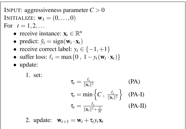
In the previous section we described a general setting for binary classification. To obtain a concrete algorithm we must determine how to initialize the weight vector w1and we must define the update rule used to modify the weight vector at the end of each round. In this section we present three variants of an online learning algorithm for binary classification. The pseudo-code for the three variants is given in Fig. 1. The vector w1 is initialized to(0, . . . ,0)for all three variants, however each variant employs a different update rule. We focus first on the simplest of the three, which on round t sets the new weight vector wt+1to be the solution to the following constrained optimization problem,
wt+1 = argmin
w∈Rn
1
2kw−wtk
2 s.t. ℓ(w;(xt,y
t)) =0. (2)
Geometrically, wt+1 is set to be the projection of wt onto the half-space of vectors which attain a
loss of zero on the current example. The resulting algorithm is passive whenever the hinge-loss is zero, that is, wt+1 =wt whenever ℓt =0. In contrast, on those rounds where the loss is
positive, the algorithm aggressively forces wt+1 to satisfy the constraint ℓ(wt+1;(xt,yt)) =0
re-gardless of the step-size required. We therefore name the algorithm Passive-Aggressive or PA for short.
The motivation for this update stems from the work of Helmbold et al. (Helmbold et al., 1999) who formalized the trade-off between the amount of progress made on each round and the amount of information retained from previous rounds. On one hand, our update requires wt+1to correctly classify the current example with a sufficiently high margin and thus progress is made. On the other hand, wt+1 must stay as close as possible to wt, thus retaining the information learned on previous
rounds.
The solution to the optimization problem in Eq. (2) has a simple closed form solution,
wt+1=wt+τtytxt where τt=
ℓt
kxtk2. (3)
We now show how this update is derived using standard tools from convex analysis (see for instance (Boyd and Vandenberghe, 2004)). Ifℓt =0 then wt itself satisfies the constraint in Eq. (2) and is
clearly the optimal solution. We therefore concentrate on the case whereℓt>0. First, we define the
Lagrangian of the optimization problem in Eq. (2) to be,
L
(w,τ) = 12kw−wtk
2 + τ 1
−yt(w·xt)
, (4)
INPUT: aggressiveness parameter C>0 INITIALIZE: w1= (0, . . . ,0)
For t=1,2, . . .
• receive instance: xt∈Rn
• predict: ˆyt =sign(wt·xt)
• receive correct label: yt∈ {−1,+1}
• suffer loss:ℓt=max{0,1−yt(wt·xt)}
• update: 1. set:
τt=kxℓttk2 (PA)
τt=min
n
C, ℓt
kxtk2 o
(PA-I)
τt=kx ℓt
tk2+2C1
(PA-II)
2. update: wt+1=wt+τtytxt
Figure 1: Three variants of the Passive-Aggressive algorithm for binary classification.
conditions (Boyd and Vandenberghe, 2004). Setting the partial derivatives of
L
with respect to the elements of w to zero gives,0 = ∇w
L
(w,τ) = w−wt−τytxt =⇒ w=wt+τytxt. (5)Plugging the above back into Eq. (4) we get,
L
(τ) = −1 2τ2
kxtk2 + τ 1−yt(wt·xt)
.
Taking the derivative of
L
(τ)with respect toτand setting it to zero, we get,0 = ∂
L
(τ)∂τ = −τkxtk2 + 1−yt(wt·xt)
=⇒ τ=1−yt(wt·xt) kxtk2 .
Since we assumed thatℓt>0 thenℓt =1−yt(w·xt). In summary, we can state a unified update for
the case whereℓt=0 and the case whereℓt>0 by settingτt=ℓt/kxtk2.
ξ, namely,
wt+1 = argmin
w∈Rn
1
2kw−wtk
2 +Cξ s.t. ℓ(w;(x
t,yt))≤ξ and ξ≥0. (6)
Here C is a positive parameter which controls the influence of the slack term on the objective func-tion. Specifically, we will show that larger values of C imply a more aggressive update step and we therefore refer to C as the aggressiveness parameter of the algorithm. We term the algorithm which results from this update PA-I .
Alternatively, we can have the objective function scale quadratically with ξ, resulting in the following constrained optimization problem,
wt+1 = argmin
w∈Rn
1
2kw−wtk
2 + Cξ2 s.t. ℓ(w;(xt,y
t))≤ξ. (7)
Note that the constraintξ≥0 which appears in Eq. (6) is no longer necessary sinceξ2 is always non-negative. We term the algorithm which results from this update PA-II . As with PA-I , C is a positive parameter which governs the degree to which the update of PA-II is aggressive. The updates of PA-I and PA-II also share the simple closed form wt+1=wt+τtytxt, where
τt=min
C, ℓt
kxtk2
(PA-I) or τt=
ℓt
kxtk2+ 1 2C
(PA-II). (8)
A detailed derivation of the PA-I and PA-II updates is provided in Appendix A. It is worth noting that the PA-II update is equivalent to increasing the dimension of each xt from n to n+T , setting
xn+t =
p
1/2C, setting the remaining T−1 new coordinates to zero, and then using the simple PA update. This technique was previously used to derive noise-tolerant online algorithms in (Klas-ner and Simon, 1995; Freund and Schapire, 1999). We do not use this observation explicitly in this paper, since it does not lead to a tighter analysis.
Up until now, we have restricted our discussion to linear predictors of the form sign(w·x). We can easily generalize any of the algorithms presented in this section using Mercer kernels. Simply note that for all three PA variants,
wt = t−1
∑
i=1
τtytxt,
and therefore,
wt·xt =
t−1
∑
i=1
τtyt(xi·xt).
The inner product on the right hand side of the above can be replaced with a general Mercer kernel
K(xi,xt)without otherwise changing our derivation. Additionally, the formal analysis presented in
the next section also holds for any kernel operator.
4. Analysis
fixed classification function of the form sign(u·x)on the same sequence. As previously mentioned, the cumulative squared hinge loss upper bounds the number of prediction mistakes. Our bounds essentially prove that, for any sequence of examples, our algorithms cannot do much worse than the best fixed predictor chosen in hindsight.
To simplify the presentation we use two abbreviations throughout this paper. As before we denote by ℓt the instantaneous loss suffered by our algorithm on round t. In addition, we denote
byℓ⋆
t the loss suffered by the arbitrary fixed predictor to which we are comparing our performance.
Formally, let u be an arbitrary vector inRn, and define
ℓt=ℓ wt;(xt,yt)
and ℓt⋆=ℓ u;(xt,yt)
. (9)
We begin with a technical lemma which facilitates the proofs in this section. With this lemma handy, we then derive loss and mistake bounds for the variants of the PA algorithm presented in the previous section.
Lemma 1 Let(x1,y1), . . . ,(xT,yT)be a sequence of examples where xt∈Rnand yt∈ {+1,−1}for
all t. Letτt be as defined by either of the three PA variants given in Fig. 1. Then using the notation
given in Eq. (9), the following bound holds for any u∈Rn,
T
∑
t=1
τt 2ℓt−τtkxtk2−2ℓ⋆t
≤ kuk2.
Proof Define∆t to be kwt−uk2− kwt+1−uk2. We prove the lemma by summing∆t over all t
in 1, . . . ,T and bounding this sum from above and below. First note that∑t∆t is a telescopic sum
which collapses to,
T
∑
t=1
∆t = T
∑
t=1
kwt−uk2− kwt+1−uk2
= kw1−uk2− kwT+1−uk2.
Using the facts that w1 is defined to be the zero vector and thatkwT+1−uk2 is non-negative, we can upper bound the right-hand side of the above bykuk2and conclude that,
T
∑
t=1
∆t ≤ kuk2. (10)
We now turn to bounding ∆t from below. If the minimum margin requirement is not violated on
round t, i.e. ℓt =0, thenτt =0 and therefore ∆t =0. We can therefore focus only on rounds for
whichℓt>0. Using the definition wt+1=wt+ytτtxt, we can write∆t as, ∆t = kwt−uk2− kwt+1−uk2
= kwt−uk2− kwt−u+ytτtxtk2
= kwt−uk2− kwt−uk2+2τtyt(wt−u)·xt+τ2tkxtk2
Since we assumed thatℓt>0 thenℓt=1−yt(wt·xt)or alternatively yt(wt·xt) =1−ℓt. In addition,
the definition of the hinge loss implies thatℓ⋆t ≥1−yt(u·xt), hence yt(u·xt)≥1−ℓ⋆t. Using these
two facts back in Eq. (11) gives,
∆t ≥ 2τt((1−ℓ⋆t)−(1−ℓt))−τ2tkxtk2
= τt 2ℓt−τtkxtk2−2ℓ⋆t
. (12)
Summing∆t over all t and comparing the lower bound of Eq. (12) with the upper bound in Eq. (10)
proves the lemma.
We first prove a loss bound for the PA algorithm in the separable case. This bound was previ-ously presented by Herbster (2001) and is analogous to the classic mistake bound for the Perceptron algorithm due to Novikoff (1962). We assume that there exists some u∈Rnsuch that yt(u·xt)>0
for all t ∈ {1, . . . ,T}. Without loss of generality we can assume that u is scaled such that that
yt(u·xt)≥1 and therefore u attains a loss of zero on all T examples in the sequence. With the
vector u at our disposal, we prove the following bound on the cumulative squared loss of PA .
Theorem 2 Let(x1,y1), . . . ,(xT,yT)be a sequence of examples where xt∈Rn, yt∈ {+1,−1}and
kxtk ≤R for all t. Assume that there exists a vector u such thatℓt⋆=0 for all t. Then, the cumulative
squared loss of PA on this sequence of examples is bounded by,
T
∑
t=1
ℓt2 ≤ kuk2R2.
Proof Sinceℓ⋆t =0 for all t, Lemma 1 implies that,
T
∑
t=1
τt 2ℓt−τtkxtk2
≤ kuk2. (13)
Using the definition ofτt for the PA algorithm in the left-hand side of the above gives,
T
∑
t=1
ℓ2t/kxtk2 ≤ kuk2.
Now using the fact thatkxtk2≤R2for all t, we get,
T
∑
t=1
ℓt2/R2 ≤ kuk2.
Multiplying both sides of this inequality by R2gives the desired bound.
the instances in the input sequence are normalized so thatkxtk2=1. Although this assumption is somewhat restrictive, it is often the case in many practical applications of classification that the instances are normalized. For instance, certain kernel operators, such as the Gaussian kernel, imply that all input instances have a unit norm. See for example (Cristianini and Shawe-Taylor, 2000).
Theorem 3 Let(x1,y1), . . . ,(xT,yT)be a sequence of examples where xt∈Rn, yt∈ {+1,−1}and
kxtk=1 for all t. Then for any vector u∈Rnthe cumulative squared loss of PA on this sequence
of examples is bounded from above by,
T
∑
t=1
ℓ2t ≤
kuk+2
q ∑T
t=1(ℓ⋆t)2
2 .
Proof In the special case wherekxtk2=1,τt andℓt are equal. Therefore, Lemma 1 gives us that, T
∑
t=1
ℓt2 ≤ kuk2+2
T
∑
t=1
ℓtℓ⋆t.
Using the Cauchy-Schwartz inequality to upper bound the right-hand side of the above inequality, and denoting
LT=
q ∑T
t=1ℓ2t and UT =
q ∑T
t=1(ℓ⋆t)2, (14)
we get that L2T ≤ kuk2+2LTUT. The largest value of LT for which this inequality is satisfied is the
larger of the two values for which this inequality holds with equality. That is, to obtain an upper bound on LT we need to find the largest root of the second degree polynomial L2T−2UTLT− kuk2,
which is,
UT+
q
UT2+kuk2. Using the fact thatpα+β≤√α+p
β, we conclude that
LT ≤ kuk+2UT. (15)
Taking the square of both sides of this inequality and plugging in the definitions of LT and UT from
Eq. (14) gives the desired bound.
Next we turn to the analysis of PA-I . The following theorem does not provide a loss bound but rather a mistake bound for the PA-I algorithm. That is, we prove a direct bound on the number of times yt6=sign(wt·xt)without using∑ℓt2as a proxy.
Theorem 4 Let(x1,y1), . . . ,(xT,yT)be a sequence of examples where xt∈Rn, yt∈ {+1,−1}and
kxtk ≤R for all t. Then, for any vector u∈Rn, the number of prediction mistakes made by PA-I on
this sequence of examples is bounded from above by,
maxR2,1/C kuk2+2C
∑
Tt=1
ℓt⋆ !
,
Proof If PA-I makes a prediction mistake on round t then ℓt ≥1. Using our assumption that
kxtk2≤R2and the definitionτt=min{ℓt/kxtk2,C}, we conclude that if a prediction mistake occurs
then it holds that,
min{1/R2,C} ≤ τtℓt.
Let M denote the number of prediction mistakes made on the entire sequence. Sinceτtℓt is always
non-negative, it holds that,
min{1/R2,C}M ≤
T
∑
t=1
τtℓt. (16)
Again using the definition ofτt, we know thatτtℓ⋆t ≤Cℓ⋆t and thatτtkxtk2≤ℓt. Plugging these two
inequalities into Lemma 1 gives,
T
∑
t=1
τtℓt ≤ kuk2+2C T
∑
t=1
ℓ⋆t. (17)
Combining Eq. (16) with Eq. (17), we conclude that,
min{1/R2,C}M ≤ kuk2+2C
T
∑
t=1
ℓ⋆t.
The theorem follows from multiplying both sides of the above by max{R2,1/C}.
Finally, we turn to the analysis of PA-II . As before, the proof of the following theorem is based on Lemma 1.
Theorem 5 Let(x1,y1), . . . ,(xT,yt)be a sequence of examples where xt ∈Rn, yt ∈ {+1,−1}and
kxtk2≤R2for all t. Then for any vector u∈Rnit holds that the cumulative squared loss of PA-II on
this sequence of examples is bounded by,
T
∑
t=1
ℓ2
t ≤
R2+ 1
2C
kuk2 +2C
T
∑
t=1 (ℓ⋆t)2
!
,
where C is the aggressiveness parameter provided to PA-II (Fig. 1) .
Proof Recall that Lemma 1 states that,
kuk2 ≥ T
∑
t=1
2τtℓt−τt2kxtk2−2τtℓ⋆t
.
Definingα=1/√2C, we subtract the non-negative term(ατt−ℓ⋆t/α)2from each summand on the
right-hand side of the above inequality, to get
kuk2 ≥ T
∑
t=1
2τtℓt−τ2tkxtk2−2τtℓt⋆−(ατt−ℓ⋆t/α)2
=
T
∑
t=1
2τtℓt−τ2tkxtk2−2τtℓt⋆−α2τt2+2τtℓt⋆−(ℓt⋆)2/α2
=
T
∑
t=1
2τtℓt−τ2t(kxtk2+α2)−(ℓ⋆t)2/α2
Plugging in the definition ofα, we obtain the following lower bound,
kuk2 ≥ T
∑
t=1
2τtℓt−τ2t
kxtk2+ 1 2C
−2C(ℓ⋆t)2
.
Using the definitionτt=ℓt/(kxtk2+1/(2C)), we can rewrite the above as,
kuk2 ≥ T
∑
t=1
ℓ2
t
kxtk2+2C1 −
2C(ℓ⋆t)2
!
.
Replacingkxtk2with its upper bound of R2and rearranging terms gives the desired bound.
We conclude this section with a brief comparison of our bounds to previously published bounds for the Perceptron algorithm. As mentioned above, the bound in Thm. 2 is equal to the bound of Novikoff (1962) for the Perceptron in the separable case. However, Thm. 2 bounds the cumulative squared hinge loss of PA , whereas Novikoff’s bound is on the number of prediction mistakes. Gentile (2002) proved a mistake bound for the Perceptron in the nonseparable case which can be compared to our mistake bound for PA-I in Thm. 4. Using our notation from Thm. 4, Gentile bounds the number of mistakes made by the Perceptron by,
R2kuk2
2 + ∑
T t=1ℓt⋆ +
r
R2kuk2∑T t=1ℓ⋆t +
R2kuk2
2
2 .
At the price of a slightly loosening this bound, we can use the inequality√a+b≤√a+√b to get
the simpler bound,
R2kuk2 + ∑T
t=1ℓ⋆t + Rkuk
q ∑T
t=1ℓt⋆.
With C=1/R2, our bound in Thm. 4 becomes,
R2kuk2 + 2
T
∑
t=1
ℓ⋆t.
Thus, our bound is inferior to Gentile’s when Rkuk< q
∑T
t=1ℓ⋆t, and even then by a factor of at
most 2.
The loss bound for PA-II in Thm. 5 can be compared with the bound of Freund and Schapire (1999) for the Perceptron algorithm. Using the notation defined in Thm. 5, Freund and Schapire bound the number of incorrect predictions made by the Perceptron by,
Rkuk+
q ∑T
t=1(ℓ⋆t)2
2 .
It can be easily verified that the bound for the PA-II algorithm given in Thm. 5 exactly equals the above bound of Freund and Schapire when C is set to kuk/(2Rp
∑t(ℓt⋆)2). Moreover, this is the
5. Regression
In this section we show that the algorithms described in Sec. 3 can be modified to deal with online regression problems. In the regression setting, every instance xt is associated with a real target
value yt ∈R, which the online algorithm tries to predict. On every round, the algorithm receives
an instance xt ∈Rn and predicts a target value ˆyt ∈Rusing its internal regression function. We
focus on the class of linear regression functions, that is, ˆyt =wt·xt where wt is the incrementally
learned vector. After making a prediction, the algorithm is given the true target value yt and suffers
an instantaneous loss. We use theε-insensitive hinge loss function:
ℓε w;(x,y)
=
0 |w·x−y| ≤ε
|w·x−y| −ε otherwise , (18)
whereε is a positive parameter which controls the sensitivity to prediction mistakes. This loss is zero when the predicted target deviates from the true target by less than ε and otherwise grows linearly with|yˆt−yt|. At the end of every round, the algorithm uses wt and the example(xt,yt)to
generate a new weight vector wt+1, which will be used to extend the prediction on the next round. We now describe how the various PA algorithms from Sec. 3 can be adapted to learn regression problems. As in the case of classification, we initialize w1 to (0, . . . ,0). On each round, the PA regression algorithm sets the new weight vector to be,
wt+1 = argmin
w∈Rn
1
2kw−wtk
2 s.t. ℓ
ε w;(xt,yt)
=0, (19)
In the binary classification setting, we gave the PA update the geometric interpretation of projecting
wt onto the linear half-space defined by the constraintℓ w;(xt,yt)
=0. For regression problems, the set{w∈Rn : ℓε(w,zt) =0} is not a half-space but rather a hyper-slab of width 2ε. Geomet-rically, the PA algorithm for regression projects wt onto this hyper-slab at the end of every round.
Using the shorthandℓt =ℓε(wt;(xt,yt)), the update given in Eq. (19) has a closed form solution
similar to that of the classification PA algorithm of the previous section, namely,
wt+1=wt+sign(yt−yˆt)τtxt where τt=ℓt/kxtk2.
We can also obtain the PA-I and PA-II variants for online regression by introducing a slack variable into the optimization problem in Eq. (19), as we did for classification in Eq. (6) and Eq. (7). The closed form solution for these updates also comes out to be wt+1=wt+sign(yt−yˆt)τtxt where τt is defined as in Eq. (8). The derivations of these closed-form updates are almost identical to that
of the classification problem in Sec. 3.
We now turn to the analysis of the three PA regression algorithms described above. We would like to show that the analysis given in Sec. 4 for the classification algorithms also holds for their regression counterparts. To do so, it suffices to show that Lemma 1 still holds for regression prob-lems. After obtaining a regression version of Lemma 1, regression versions of Thm. 2 through Thm. 5 follow as immediate corollaries.
Lemma 6 Let(x1,y1), . . . ,(xT,yT)be an arbitrary sequence of examples, where xt∈Rnand yt∈R
for all t. Letτt be as defined in either of the three PA variants for regression problems. Then using
the notation given in Eq. (9), the following bound holds for any u∈Rn,
T
∑
t=1
τt 2ℓt−τtkxtk2−2ℓ⋆t
Proof The proof of this lemma follows that of Lemma 1 and therefore subtleties which were
dis-cussed in detail in that proof are omitted here. Again, we use the definition
∆t =kwt−uk2− kwt+1−uk2 and the same argument used in Lemma 1 implies that,
T
∑
t=1
∆t ≤ kuk2,
We focus our attention on bounding ∆t from below on those rounds where ∆t 6=0. Using the
recursive definition of wt+1, we rewrite∆t as,
∆t = kwt−uk2− kwt−u+sign(yt−yˆt)τtxtk2
= −sign(yt−yˆt)2τt(wt−u)·xt −τt2kxtk2
We now add and subtract the term sign(yt−yˆt)2τtyt from the right-hand side above to get the bound,
∆t ≥ −sign(yt−yˆt)2τt(wt·xt−yt) +sign(yt−yˆt)2τt(u·xt−yt)−τ2tkxtk2. (20)
Since wt·xt=yˆt, we have that−sign(yt−yˆt)(wt·xt−yt) =|wt·xt−yt|. We only need to consider
the case where∆t 6=0, soℓt=|wt·xt−yt| −εand we can rewrite the bound in Eq. (20) as,
∆t ≥ 2τt(ℓt+ε) +sign(yt−yˆt)2τt(u·xt−yt)−τ2tkxtk2.
We also know that sign(yt−yˆt)(u·xt−yt)≥ −|u·xt−yt|and that−|u·xt−yt| ≥ −(ℓ⋆t +ε). This
enables us to further bound,
∆t ≥ 2τt(ℓt+ε)−2τt(ℓ⋆t +ε)−τ2tkxtk2 = τt(2ℓt−τtkxtk2−2ℓ⋆t).
Summing the above over all t and comparing to the upper bound discussed in the beginning of this proof proves the lemma.
6. Uniclass Prediction
In this section we present PA algorithms for the uniclass prediction problem. This task involves predicting a sequence of vectors y1,y2,··· where yt∈Rn. Uniclass prediction is fundamentally
dif-ferent than classification and regression as the algorithm makes predictions without first observing any external input (such as the instance xt). Specifically, the algorithm maintains in its memory a
vector wt ∈Rnand simply predicts the next element of the sequence to be wt. After extending this
prediction, the next element in the sequence is revealed and an instantaneous loss is suffered. We measure loss using the followingε-insensitive loss function:
ℓε(w; y) =
0 kw−yk ≤ε
kw−yk −ε otherwise . (21)
distance between the prediction and the true vector. At the end of each round wt is updated in order
to have a potentially more accurate prediction on where the next element in the sequence will fall. Equivalently, we can think of uniclass prediction as the task of finding a center-point w such that as many vectors in the sequence fall within a radius ofεfrom w. At the end of this section we discuss a generalization of this problem, where the radiusεis also determined by the algorithm.
As before, we initialize w1= (0, . . . ,0). Beginning with the PA algorithm, we define the update for the uniclass prediction algorithm to be,
wt+1 = argmin
w∈Rn
1
2kw−wtk
2 s.t. ℓ
ε(w; yt) =0, (22)
Geometrically, wt+1is set to be the projection of wt onto a ball of radiusεabout yt. We now show
that the closed form solution of this optimization problem turns out to be,
wt+1 =
1− ℓt
kwt−ytk
wt +
ℓt
kwt−ytk
yt. (23)
First, we rewrite the above equation and express wt+1by,
wt+1=wt+τt
yt−wt
kyt−wtk
, (24)
whereτt =ℓt. In the Uniclass problem the KKT conditions are both sufficient and necessary for
optimality. Therefore, we prove that Eq. (24) is the minimizer of Eq. (22) by verifying that the KKT conditions indeed hold. The Lagrangian of Eq. (22) is,
L
(w,τ) = 12kw−wtk
2+τ(kw−y
tk −ε), (25)
whereτ≥0 is a Lagrange multiplier. Differentiating with respect to the elements of w and setting these partial derivatives to zero, we get the first KKT condition, stating that at the optimum(w,τ) must satisfy the equality,
0 = ∇w
L
(w,τ) = w−wt+τw−yt
kw−ytk. (26)
In addition, an optimal solution must satisfy the conditionsτ≥0 and,
τ(kw−ytk −ε) = 0. (27)
Clearly, τt ≥0. Therefore, to show that wt+1 is the optimum of Eq. (22) it suffices to prove that (wt+1,τt)satisfies Eq. (26) and Eq. (27). These equalities trivially hold ifℓt=0 and therefore from
now on we assume thatℓt >0. Plugging the values w=wt+1andτ=τt in the right-hand side of
Eq. (26) gives,
wt+1−wt+τt
wt+1−yt
kwt+1−ytk = τt
yt−wt
kyt−wtk+
wt+1−yt
kwt+1−ytk
. (28)
Note that,
wt+1−yt = wt+τt
yt−wt
kyt−wtk−
yt = (wt−yt)
1−τt
1 kyt−wtk
= wt−yt kwt−ytk
(kwt−ytk −τt) = ε
kwt−ytk
Combining Eq. (29) with Eq. (28) we get that,
wt+1−wt+τt
wt+1−yt kwt+1−ytk
= 0,
and thus Eq. (26) holds for(wt+1,τt). Similarly,
kwt+1−ytk −ε = ε−ε = 0,
and thus Eq. (27) also holds. In summary, we have shown that the KKT optimality conditions hold for(wt+1,τt)and therefore Eq. (24) gives the desired closed-form update.
To obtain uniclass versions of PA-I and PA-II , we add a slack variable to the optimization problem in Eq. (22) in the same way as we did in Eq. (6) and Eq. (7) for the classification algorithms. Namely, the update for PA-I is defined by,
wt+1 = argmin
w∈Rn
1
2kw−wtk
2+Cξ s.t.
kw−ytk ≤ε+ξ, ξ≥0, (30)
and the update for PA-II is,
wt+1 = argmin
w∈Rn
1
2kw−wtk
2+Cξ2 s.t.
kw−ytk ≤ε+ξ.
The closed form for these updates can be derived using the same technique as we used for deriving the PA update. The final outcome is that both PA-I and PA-II share the form of update given in Eq. (24), withτt set to be,
τt=min{C, ℓt } (PA-I) or τt=
ℓt
1+ 1 2C
(PA-II).
We can extend the analysis of the three PA variants from Sec. 4 to the case of uniclass prediction. We do so by proving a uniclass version of Lemma 1. After proving this lemma, we discuss an additional technical difficulty which needs to be addressed so that Thm. 2 through Thm. 5 carry over smoothly to the uniclass case.
Lemma 7 Let y1, . . . ,yT be an arbitrary sequence of vectors, where yt ∈Rnfor all t. Letτt be as
defined in either of the three PA variants for uniclass prediction. Then using the notation given in
Eq. (9), the following bound holds for any u∈Rn,
T
∑
t=1
τt(2ℓt−τt−2ℓ⋆t) ≤ kuk2.
Proof We prove this lemma in much the same way as we did Lemma 1. We again use the definition, ∆t=kwt−uk2− kwt+1−uk2, along with the fact stated in Eq. (10) that
T
∑
t=1
We now focus our attention on bounding∆t from below on those rounds where ∆t 6=0. Using the
recursive definition of wt+1, we rewrite∆t as, ∆t = kwt−uk2−
1− τt
kwt−ytk
wt +
τ
t
kwt−ytk
yt−u
2
= kwt−uk2−
(wt−u) +
τ
t
kwt−ytk
(yt−wt)
2
= −2
τ
t
kwt−ytk
(wt−u)·(yt−wt)−τ2t.
We now add and subtract yt from the term(wt−u)above to get,
∆t = −2
τ
t
kwt−ytk
(wt−yt+yt−u)·(yt−wt)−τt2 = 2τtkwt−ytk −2
τ
t
kwt−ytk
(yt−u)·(yt−wt)−τ2t.
Now, using the Cauchy-Schwartz inequality on the term(yt−u)·(yt−wt), we can bound,
∆t ≥ 2τtkwt−ytk −2τtkyt−uk −τ2t.
We now add and subtract 2τtεfrom the right-hand side of the above, to get,
∆t ≥ 2τt(kwt−ytk −ε)−2τt(kyt−uk −ε)−τ2t.
Since we are dealing with the case where ℓt >0, it holds thatℓt =kwt−ytk −ε. By definition,
ℓ⋆t ≥ ku−ytk −ε. Using these two facts, we get,
∆t ≥ 2τtℓt−2τtℓ⋆t −τ2t.
Summing the above inequality over all t and comparing the result to the upper bound in Eq. (10) gives the bound stated in the lemma.
As mentioned above, there remains one more technical obstacle which stands in the way of applying Thm. 2 through Thm. 5 to the uniclass case. This difficulty stems from the fact xt is not
defined in the uniclass whereas the termkxk2appears in the theorems. This issue is easily resolved by setting xt in the uniclass case to be an arbitrary vector of a unit length, namelykxtk2=1. This
technical modification enables us to write τt asℓt/kxtk2 in the uniclass PA algorithm, as in the
classification case. Similarly, τt can be defined as in the classification case for PA-I and PA-II .
Now Thm. 2 through Thm. 5 can be applied verbatim to the uniclass PA algorithms.
be arbitrarily large and does not appear in our analysis. Typically, we will think of B as being far greater than any conceivable value ofε. Our goal is now to incrementally find wtandεt such that,
kwt−ytk ≤εt, (31)
as often as possible. Additionally, we would like εt to stay relatively small, since an extremely
large value ofεt would solve the problem in a trivial way. We do so by reducing this problem to a
different uniclass problem where the radius is fixed and where yt is inRn+1. That is, by adding an
additional dimension to the problem, we can learnεusing the same machinery developed for fixed-radius uniclass problems. The reduction stems from the observation that Eq. (31) can be written equivalently as,
kwt−ytk2+ (B2−ε2t) ≤ B2. (32)
If we were to concatenate a 0 to the end of every yt (thus increasing its dimension to n+1) and
if we considered the n+1’th coordinate of wt to be equivalent to
p
B2−ε2
t, then Eq. (32) simply
becomeskwt−ytk2 ≤ B2. Our problem has reduced to a fixed-radius uniclass problem where the radius is set to B. w1,n+1should be initialized to B, which is equivalent to initializingε1=0. On each round,εt can be extracted from wt by,
εt =
q
B2−w2
t,n+1.
Since wt+1,n+1 is defined to be a convex combination of wt,n+1and yt,n+1(where the latter equals zero), then wt,n+1 is bounded in(0,B]for all t and can only decrease from round to round. This means that the radiusεt is always well defined and can only increase with t. Since the radius is
initialized to zero and is now one of the learned parameters, the algorithm has a natural tendency to favor small radii. Let u denote the center of a fixed uniclass predictor and letεdenote its radius. Then the reduction described above enables us to prove loss bounds similar to those presented in Sec. 4, withkuk2replaced bykuk2+ε2.
7. Multiclass Problems
We now address more complex decision problems. We first adapt the binary classification algo-rithms described in Sec. 3 to the task of multiclass multilabel classification. In this setting, every instance is associated with a set of labels Yt. For concreteness we assume that there are k different
possible labels and denote the set of all possible labels by
Y
={1, . . . ,k}. For every instance xt, theset of relevant labels Yt is therefore a subset of
Y
. We say that label y is relevant to the instance xt ify∈Yt. This setting is often discussed in text categorization applications (see for instance (Schapire
and Singer, 2000)) where xt represents a document and Yt is the set of topics which are relevant to
the document and is chosen from a predefined collection of topics. The special case where there is only a single relevant topic for each instance is typically referred to as multiclass single-label classification or multiclass categorization for short. As discussed below, our adaptation of the PA variants to multiclass multilabel settings encompasses the single-label setting as a special case.
As in the previous sections, the algorithm receives instances x1,x2, . . .in a sequential manner where each xt belongs to an instance space
X
. Upon receiving an instance, the algorithm outputsa score for each of the k labels in
Y
. That is, the algorithm’s prediction is a vector in Rk whereflexible than predicting the set of relevant labels Yt. Special purpose learning algorithms such as
AdaBoost.MR (Schapire and Singer, 1998) and adaptations of support vector machines (Crammer and Singer, 2003a) have been devised for the task of label ranking. Here we describe a reduction from online label ranking to online binary classification that deems label ranking as simple as binary prediction. We note that in the case of multiclass single-label classification, the prediction of the algorithm is simply set to be the label with the highest score.
For a pair of labels r,s∈
Y
, if the score assigned by the algorithm to label r is greater than the score assigned to label s, we say that label r is ranked higher than label s. The goal of the algorithm is to rank every relevant label above every irrelevant label. Assume that we are provided with a set of d features φ1, . . . ,φd where each featureφj is a mapping fromX
×Y
to the reals. We denotebyΦ(x,y) = (φ1(x,y), . . . ,φd(x,y))the vector formed by concatenating the outputs of the features,
when each feature is applied to the pair(x,y). The label ranking function discussed in this section is parameterized by a weight vector, w∈Rd. On round t, the prediction of the algorithm is the
k-dimensional vector,
(wt·Φ(xt,1)), . . . ,(wt·Φ(xt,k)).
We motivate our construction with an example from the domain of text categorization. We describe a variant of the Term Frequency - Inverse Document Frequency (TF-IDF) representation of docu-ments (Rocchio, 1971; Salton and Buckley, 1988). Each featureφjcorresponds to a different word,
denoted µj. Given a corpus of documents S, for every x∈S and for every potential topic y, the
featureφj(x,y)is defined to be,
φj(x,y) = TF(µj,x)·log
|S|
DF(µj,y)
,
where TF(µj,x) is the number of times µj appears in x and DF(µj,y) is the number of times µj
appears in all of the documents in S which are not labeled by y. The valueφjgrows in proportion to
the frequency of µjin the document x but is dampened if µj is a frequent word for topics other than
y. In the context of this paper, the important point is that each feature is label-dependent.
After making its prediction (a ranking of the labels), the algorithm receives the correct set of relevant labels Yt. We define the margin attained by the algorithm on round t for the example(xt,Yt)
as,
γ wt;(xt,Yt)
= min
r∈Yt
wt·Φ(xt,r) − max
s6∈Yt
wt·Φ(xt,s).
This definition generalizes the definition of margin for binary classification and was employed by both single-label and multilabel learning algorithms for support vector machines (Vapnik, 1998; Weston and Watkins, 1999; Elisseeff and Weston, 2001; Crammer and Singer, 2003a). In words, the margin is the difference between the score of the lowest ranked relevant label and the score of the highest ranked irrelevant label. The margin is positive only if all of the relevant labels are ranked higher than all of the irrelevant labels. However, in the spirit of binary classification, we are not satisfied by a mere positive margin as we require the margin of every prediction to be at least 1. After receiving Yt, we suffer an instantaneous loss defined by the following hinge-loss function,
ℓMC w;(x,Y)
=
0 γ w;(x,Y)
≥1 1−γ w;(x,Y)
As in the previous sections, we useℓt as an abbreviation forℓMC wt;(xt,Yt)
. If an irrelevant label is ranked higher than a relevant label, thenℓ2
t attains a value greater than 1. Therefore,∑Tt=1ℓt2upper
bounds the number of multiclass prediction mistakes made on rounds 1 through T .
One way of updating the weight vector wt is to mimic the derivation of the PA algorithm for
binary classification defined in Sec. 3 and to set
wt+1 = argmin
w∈Rd
1
2kw−wtk
2 s.t. ℓ
MC(w;(xt,Yt)) =0. (34)
Satisfying the single constraint in the optimization problem above is equivalent to satisfying the following set of linear constraints,
∀r∈Yt ∀s6∈Yt w·Φ(xt,r)−w·Φ(xt,s) ≥ 1. (35)
However, instead of attempting to satisfy all of the|
Y
t| ×(k− |Y
t|)constraints above we focus onlyon the single constraint which is violated the most by wt. We show in the sequel that we can still
prove a cumulative loss bound for this simplified version of the update. We note that satisfying all of these constraints simultaneously leads to the online algorithm presented in (Crammer and Singer, 2003a). Their online update is more involved and computationally expensive, and moreover, their analysis only covers the realizable case.
Formally, let rt denote the lowest ranked relevant label and let st denote the highest ranked
irrelevant label on round t. That is,
rt = argmin r∈Yt
wt·Φ(xt,r) and st = argmax s6∈Yt
wt·Φ(xt,s). (36)
The single constraint that we choose to satisfy is w·Φ(xt,rt)−w·Φ(xt,st)≥1 and thus wt+1is set to be the solution of the following simplified constrained optimization problem,
wt+1 = argmin
w
1
2kw−wtk
2 s.t. w
·(Φ(xt,rt)−Φ(xt,st)) ≥ 1. (37)
The apparent benefit of this simplification lies in the fact that Eq. (37) has a closed form solution. To draw the connection between the multilabel setting and binary classification, we can think of the vectorΦ(xt,rt)−Φ(xt,st)as a virtual instance of a binary classification problem with a label of
+1. With this reduction in mind, Eq. (37) becomes equivalent to Eq. (2). Therefore, the closed form solution of Eq. (37) is
wt+1 = wt+τt(Φ(xt,rt)−Φ(xt,st)). (38)
with,
τt =
ℓt
kΦ(xt,rt)−Φ(xt,st)k2
.
Although we are essentially neglecting all but two labels on each step of the multiclass update, we can still obtain multiclass cumulative loss bounds. The key observation in our analysis it that,
ℓMC wt;(xt,Yt)
= ℓ wt;(Φ(xt,rt)−Φ(xt,st),+1)
.
the multiclass PA algorithm. To do so we need to cast the assumption that for all t it holds that
kΦ(xt,rt)−Φ(xt,st)k ≤R. This bound can immediately be converted into a bound on the norm
of the feature set sincekΦ(xt,rt)−Φ(xt,st)k ≤ kΦ(xt,rt)k+kΦ(xt,st)k. Thus, if the norm of the
mapping Φ(xt,r) is bounded for all t and r then so is kΦ(xt,rt)−Φ(xt,st)k. In particular, if we
assume thatkΦ(xt,r)k ≤R/2 for all t and r we obtain the following corollary.
Corollary 8 Let(x1,Y1), . . . ,(xT,YT)be a sequence of examples with xt∈Rnand YT ⊆ {1, . . . ,k}.
LetΦbe a mappingΦ:
X
×Y
→Rd such thatkΦ(xt,r)k ≤R/2 for all t and r. Assume that there
exists a vector u such thatℓ(u;(xt,Yt)) =0 for all t. Then, the cumulative squared loss attained by
the multiclass multilabel PA algorithm is bounded from above by,
T
∑
t=1
ℓt2 ≤ R2kuk2.
Similarly, we can obtain multiclass versions of PA-I and PA-II by using the update rule in Eq. (38) but settingτt to be either,
τt = min
C, ℓt
kΦ(xt,rt)−Φ(xt,st)k2
or τt =
ℓt
kΦ(xt,rt)−Φ(xt,st)k2+2C1
,
respectively. The analysis of PA-I and PA-II in Thms. 4-5 also carries over from the binary case to the multilabel case in the same way.
Multi-prototype Classification In the above discussion we assumed that the feature vectorΦ(x,y) is label-dependent and used a single weight vector w to form the ranking function. However, in many applications of multiclass classification this setup is somewhat unnatural. Many times, there is a single natural representation for every instance rather than multiple feature representations for each individual class. For example, in optical character recognition problems (OCR) an instance can be a gray-scale image of the character and the goal is to output the content of this image. In this example, it is difficult to find a good set of label-dependent features.
The common construction in such settings is to assume that each instance is a vector inRnand to associate a different weight vector (often referred to as prototype) with each of the k labels (Vapnik, 1998; Weston and Watkins, 1999; Crammer and Singer, 2001). That is, the multiclass predictor is now parameterized by w1t, . . . ,wkt, where wtr∈Rn. The output of the predictor is defined to be,
(w1t ·xt), . . . ,(wkt ·xt)
.
To distinguish this setting from the previous one we refer to this setting as the multi-prototype mul-ticlass setting and to the previous one as the single-prototype mulmul-ticlass setting. We now describe a reduction from the multi-prototype setting to the single-prototype one which enables us to use all of the multiclass algorithms discussed above in the multi-prototype setting as well. To obtain the desired reduction, we must define the feature vector representationΦ(x,y)induced by the instance label pair(x,y). We defineΦ(x,y)to be a k·n dimensional vector which is composed of k blocks of
size n. All blocks but the y’th block ofΦ(x,y)are set to be the zero vector while the y’th block is set to be x. Applying a single prototype multiclass algorithm to this problem produces a weight vector
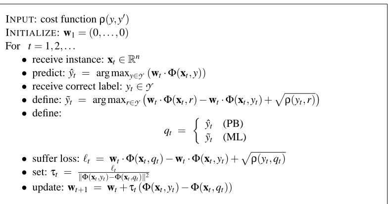
INPUT: cost functionρ(y,y′)
INITIALIZE: w1= (0, . . . ,0) For t=1,2, . . .
• receive instance: xt∈Rn
• predict: ˆyt = arg maxy∈Y (wt·Φ(xt,y))
• receive correct label: yt∈
Y
• define: ˜yt = arg maxr∈Y wt·Φ(xt,r)−wt·Φ(xt,yt) +
p ρ(yt,r)
• define:
qt =
ˆ
yt (PB)
˜
yt (ML)
• suffer loss:ℓt = wt·Φ(xt,qt)−wt·Φ(xt,yt) +
p
ρ(yt,qt)
• set:τt = kΦ(x ℓt
t,yt)−Φ(xt,qt)k2
• update: wt+1 = wt+τt(Φ(xt,yt)−Φ(xt,qt))
Figure 2: The prediction-based (PB) and max-loss (ML) passive-aggressive updates for cost-sensitive multiclass problems.
of k blocks of size n and denote block r by wrt. By construction, we get that wt·Φ(xt,r) =wrt·xt.
Equipped with this construction we can use verbatim any single-prototype algorithm as a proxy for the multi-prototype variant. Namely, on round t we find the pair of indices rt,st which corresponds
to the largest violation of the margin constraints,
rt = argmin
r∈Yt
wt·Φ(xt,r) = argmin r∈Yt
wrt·xt ,
st = argmax
s6∈Yt
wt·Φ(xt,s) = argmax s6∈Yt
wst·xt. (39)
Unraveling the single-prototype notion of margin and casting it as a multi-prototype one we get that the loss in the multi-prototype case amounts to,
ℓ w1t, . . . ,wtk;(xt,Yt)
=
0 wrt
t ·xt−wstt·xt ≥1
1−wrt
t ·xt+wtst·xt otherwise
. (40)
Furthermore, applying the same reduction to the update scheme we get that the resulting multi-prototype update is,
wrt
t+1=w
rt
t+1+τtxt and w
st
t+1=w
st
t+1−τtxt. (41) For the PA algorithm, the value ofτt is the ratio of the loss, as given by Eq. (40), and the squared
norm ofΦ(xt,rt)−Φ(xt,st). By construction, this vector has k−2 blocks whose elements are zeros
and two blocks that are equal to xt and−xt. Since the two non-zero blocks are non-overlapping we
get that,
kΦ(xt,rt)−Φ(xt,st)k2=kxtk2+k −xtk2=2kxtk2.
8. Cost-Sensitive Multiclass Classification
Cost-sensitive multiclass classification is a variant of the multiclass single-label classification setting discussed in the previous section. Namely, each instance xt is associated with a single correct label
yt∈
Y
and the prediction extended by the online algorithm is simply,ˆ
yt = argmax y∈Y
(wt·Φ(xt,y)). (42)
A prediction mistake occurs if yt6=yˆt, however in the cost-sensitive setting different mistakes incur
different levels of cost. Specifically, for every pair of labels(y,y′)there is a costρ(y,y′)associated with predicting y′ when the correct label is y. The cost functionρis defined by the user and takes non-negative values. We assume thatρ(y,y) =0 for all y∈
Y
and thatρ(y,y′)≥0 whenever y6=y′. The goal of the algorithm is to minimize the cumulative cost suffered on a sequence of examples, namely to minimize∑ρ(yt,yˆt).The multiclass PA algorithms discussed above can be adapted to this task by incorporating the cost function into the online update. Recall that we began the derivation of the multiclass PA update by defining a set of margin constraints in Eq. (35), and on every round we focused our attention on satisfying only one of these constraints. We repeat this idea here while incorporating the cost function into the margin constraints. Specifically, on every online round we would like for the following constraints to hold,
∀r∈ {
Y
\yt} wt·Φ(xt,yt)−wt·Φ(xt,r) ≥p
ρ(yt,r). (43)
The reason for using the square root function in the equation above will be justified shortly. As mentioned above, the online update focuses on a single constraint out of the|
Y
| −1 constraints in Eq. (43). We will describe and analyze two different ways to choose this single constraint, which lead to two different online updates for cost-sensitive classification. The two update techniques are called the prediction-based update and the max-loss update. Pseudo-code for these two updates is presented in Fig. 2. They share an almost identical analysis and may seem very similar at first, however each update possesses unique qualities. We discuss the significance of each update at the end of this section.The prediction-based update focuses on the single constraint in Eq. (43) which corresponds to the predicted label ˆyt. Concretely, this update sets wt+1to be the solution to the following optimiza-tion problem,
wt+1 = argmin
w∈Rn
1
2kw−wtk
2 s.t. wt
·Φ(xt,yt)−wt·Φ(xt,yˆt) ≥
p
ρ(yt,yˆt), (44)
where ˆyt is defined in Eq. (42). This update closely resembles the multiclass update given in
Eq. (37). Define the cost sensitive loss for the prediction-based update to be,
ℓPB w;(x,y)
= w·Φ(x,yˆ)−w·Φ(x,y) +pρ(y,yˆ). (45)
Note that this loss equals zero if and only if a correct prediction was made, namely if ˆyt =yt. On
the other hand, if a prediction mistake occurred it means that wt ranked ˆyt higher than yt, thus,
p
ρ(yt,yˆt) ≤ wt·Φ(xt,yˆt)−wt·Φ(xt,yt) +
p