Learning Gradients: Predictive Models that Infer Geometry and Statistical Dependence

Learning Gradients: Predictive Models that Infer Geometry and

Statistical Dependence

Qiang Wu [email protected]

Department of Mathematics Michigan State University East Lansing, MI 48824, USA

Justin Guinney [email protected]

Sage Bionetworks

Fred Hutchinson Cancer Research Center Seattle, WA 98109, USA

Mauro Maggioni∗ [email protected]

Sayan Mukherjee† [email protected]

Departments of Mathematics and Statistical Science Duke University

Durham, NC 27708, USA

Editor: Marina Meila

Abstract

The problems of dimension reduction and inference of statistical dependence are addressed by the modeling framework of learning gradients. The models we propose hold for Euclidean spaces as well as the manifold setting. The central quantity in this approach is an estimate of the gradient of the regression or classification function. Two quadratic forms are constructed from gradient estimates: the gradient outer product and gradient based diffusion maps. The first quantity can be used for supervised dimension reduction on manifolds as well as inference of a graphical model encoding dependencies that are predictive of a response variable. The second quantity can be used for nonlinear projections that incorporate both the geometric structure of the manifold as well as variation of the response variable on the manifold. We relate the gradient outer product to standard statistical quantities such as covariances and provide a simple and precise comparison of a variety of supervised dimensionality reduction methods. We provide rates of convergence for both inference of informative directions as well as inference of a graphical model of variable dependencies.

Keywords: gradient estimates, manifold learning, graphical models, inverse regression, dimension reduction, gradient diffusion maps

1. Introduction

The problem of developing predictive models given data from high-dimensional physical and bi-ological systems is central to many fields such as computational biology. A premise in modeling natural phenomena of this type is that data generated by measuring thousands of variables lie on or near a low-dimensional manifold. This hearkens to the central idea of reducing data to only relevant

∗. Also in the Department of Computer Science.

information. This idea was fundamental to the paradigm of Fisher (1922) and goes back at least to Adcock (1878) and Edgeworth (1884). For an excellent review of this program see Cook (2007). In this paper we examine how this paradigm can be used to infer geometry of the data as well as statistical dependencies relevant to prediction.

The modern reprise of this program has been developed in the broad areas of manifold learn-ing and simultaneous dimension reduction and regression. Manifold learnlearn-ing has focused on the problem of projecting high-dimensional data onto a few directions or dimensions while respect-ing local structure and distances. A variety of unsupervised methods have been proposed for this problem (Tenenbaum et al., 2000; Roweis and Saul, 2000; Belkin and Niyogi, 2003; Donoho and Grimes, 2003). Simultaneous dimension reduction and regression considers the problem of finding directions that are informative with respect to predicting the response variable. These methods can be summarized by three categories: (1) methods based on inverse regression (Li, 1991; Cook and Weisberg, 1991; Fukumizu et al., 2005; Wu et al., 2007), (2) methods based on gradients of the regression function (Xia et al., 2002; Mukherjee and Zhou, 2006; Mukherjee and Wu, 2006), (3) methods based on combining local classifiers (Hastie and Tibshirani, 1996; Sugiyama, 2007). Our focus is on the supervised problem. However, we will use the core idea in manifold learning, local estimation.

We first illustrate with a simple example how gradient information can be used for supervised dimension reduction. Both linear projections as well as nonlinear embeddings based on gradient estimates are used for supervised dimension reduction. In both approaches the importance of using the response variable is highlighted.

The main contributions in this paper consist of (1) development of gradient based diffusion maps, (2) precise statistical relations between the above three categories of supervised dimension reduction methods, (3) inference of graphical models or conditional independence structure given gradient estimates, (4) rates of convergence of the estimated graphical model. The rate of con-vergence depends on a geometric quantity, the intrinsic dimension of the gradient on the manifold supporting the data, rather than the sparsity of the graph.

2. A Statistical Foundation for Learning Gradients

The problem of regression can be summarized as estimating the function

fr(x) =E(Y|X=x)

from data D=_{Li = (Yi,Xi)}ni=1 where Xi is a vector in a p-dimensional compact metric space

X _∈

X

i∈R is a real valued output. Typically the data are drawn iid from a joint distribution, Liiid∼ρ(X,Y)thus specifying a model

yi= fr(xi) +εi

with εi drawn iid from a specified noise model. We define ρX as the marginal distribution of the

explanatory variables.

In this paper we will explain how inference of the gradient of the regression function

∇fr=

∂

fr ∂x1, ...,

∂fr ∂xp

provides information on the geometry and statistical dependencies relevant to predicting the re-sponse variable given the explanatory variables. Our work is motivated by the following ideas. The gradient is a local concept as it measures local changes of a function. Integrating informa-tion encoded by the gradient allows for inference of the geometric structure in the data relevant to the response. We will explore two approaches to integrate this local information. The first ap-proach is averaging local gradient estimates and motivates the study of the gradient outer product (GOP) matrix. The GOP can be used to motivate a variety of linear supervised dimension reduction formulations. The GOP can also be considered as a covariance matrix and used for inference of conditional dependence between predictive explanatory variables. The second approach is to paste local gradient estimates together. This motivates the study of gradient based diffusion maps (GDM). This operator can be used for nonlinear supervised dimension reduction by embedding the support of the marginal distribution onto a much lower dimensional manifold that varies with respect to the response.

The gradient outer productΓis a p_×p matrix with elements

Γi j=

∂

fr ∂xi,

∂fr ∂xj

L2

ρ_X

,

where ρX is the marginal distribution of the explanatory variables and L

2

ρX is the space of square

integrable functions with respect to the measureρX. Using the notation a⊗b=ab

T _{for a,b∈R}p_,

we can write

Γ=E(∇fr⊗∇fr).

This matrix provides global information about the predictive geometry of the data (developed in Section 2.2) as well as inference of conditional independence between variables (developed in Sec-tion 5). The GOP is meaningful in both the Euclidean as well as the manifold setting where the marginal distribution ρX is concentrated on a much lower dimensional manifold

M

dM (developed in Section 4.1.2).

Since the GOP is a global quantity and is constructed by averaging the gradient over the marginal distribution of the data it cannot isolate local information or local geometry. This global summary of the joint distribution is advantageous in statistical analyses where global inferences are desired: global predictive factors comprised of the explanatory variables or global estimates of statistical de-pendence between explanatory variables. It is problematic to use a global summary for constructing a nonlinear projection or embedding that captures the local predictive geometry on the marginal distribution.

Random walks or diffusions on manifolds and graphs have been used for a variety of nonlinear dimension reduction or manifold embedding procedures (Belkin and Niyogi, 2003, 2004; Szummer and Jaakkola, 2001; Coifman et al., 2005a,b). Our basic idea is to use local gradient information to construct a random walk on a graph or manifold based on the ideas of diffusion analysis and diffusion geometry (Coifman and Lafon, 2006; Coifman and Maggioni, 2006). The central quantity in diffusion based approaches is the definition of a diffusion operator L based on a similarity metric

Wi j between two points xiand xj. A commonly used diffusion operator is the graph Laplacian

L=I₋D−1/2W D−1/2, where Dii=

∑

Wi j.

We propose the following similarity metric called the gradient based diffusion map (GDM) to smoothly paste together local gradient estimates

Wi j=Wf(xi,xj) =exp −k

xi−xjk2

σ1 −

|1

2(∇fr(xi) +∇fr(xj))·(xi−xj)|2

σ2

!

.

In the above equation the first termkxi−xjk2encodes the local geometry of the marginal distribution and the second term pastes together gradient estimates between neighboring points. The first term is used in unsupervised dimension reduction methods such as Laplacian eigenmaps or diffusion maps (Belkin and Niyogi, 2003). The second term can be interpreted as a diffusion map on the function values, the approximation is due to a first order Taylor expansion

1

2(∇fr(xi) +∇fr(xj))·(xi−xj)≈ fr(xi)−fr(xj) if xi≈xj.

A related similarity was briefly mentioned in Coifman et al. (2005b) and used in Szlam et al. (2008) in the context of semi-supervised learning. In Section 4.2 we study this nonlinear projection method under the assumption that the marginal distribution is concentrated on a much lower dimensional manifold

M

2.1 Illustration of Linear Projections and Nonlinear Embeddings

The simple example in this section fixes the differences between linear projections and nonlinear embeddings using either diffusion maps or gradient based diffusion maps. The marginal distribution is uniform on the following manifold

X1=t cos(t), X2=70h, X3=t sin(t)where t= 3π

2 (1+2θ),θ∈[0,1],h∈[0,1],

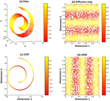
and the regression function is Y =sin(5πθ), see Figure 1(a). In this example a two dimensional manifold is embedded inR3 and the variation of the response variable can be embedded onto one dimension. The points in Figure 1(a) are the points on the manifold and the false color signifies the function value at these points. In Figure 1(b) the data is embedded in two dimensions using diffusion maps with the function values displayed in false color. It is clear that the direction of greatest variation is X2 which corresponds to h. It is not the direction along which the regression function has greatest variation. In Figure 1(c) the data is projected onto two axes using the GOP approach and we see that the relevant dimensions X1,X3 are recovered. This example also shows that linear dimension reduction may still make sense in the manifold setting. In Figure 1(d) the data is embedded using gradient based diffusion maps and we capture the directionθin which the data varies with respect to the regression function.

2.2 Gradient Outer Product Matrix and Dimension Reduction

In the case of linear supervised dimension reduction we assume the following semi-parametric model holds

Y =fr(X) +ε=g(bT1X, . . . ,bTdX) +ε, (1)

whereεis noise and B= (bT₁, ...,bT

−10 0 10 20 0 50 100 −15 −10 −5 0 5 10 15 x (a) Data y z

0 0.2 0.4 0.6 0.8 1

0 0.1 0.2 0.3 0.4 0.5 0.6 0.7 0.8 0.9 1 Dimension 1 Dimension 2

(b) Diffusion map

−10 0 10 20

−15 −10 −5 0 5 10 15 Dimension 1 Dimension 2 (c) GOP

0 0.2 0.4 0.6 0.8 1

0 0.1 0.2 0.3 0.4 0.5 0.6 0.7 0.8 0.9 1 Dimension 1 Dimension 2 (d) GDM −0.8 −0.6 −0.4 −0.2 0 0.2 0.4 0.6 0.8 −0.8 −0.6 −0.4 −0.2 0 0.2 0.4 0.6 0.8 −0.8 −0.6 −0.4 −0.2 0 0.2 0.4 0.6 0.8 −0.8 −0.6 −0.4 −0.2 0 0.2 0.4 0.6 0.8

Figure 1: (a) Plot of the original three dimensional data with the color of the point correspond-ing to the function value; (b) Embeddcorrespond-ing the data onto two dimensions uscorrespond-ing diffusion maps, here dimensions 1 and 2 corresponds to h andθrespectively; (c) Projection of the data onto two dimensions using gradient based dimension reduction, here dimensions 1 and 2 corresponds to x and z respectively; (d) Embedding the data onto two dimensions using gradient based diffusion maps, here dimensions 1 and 2 corresponds toθand h respectively.

and dimension reduction becomes the central problem in finding an accurate regression model. In the following we develop theory relating the gradient of the regression function to the above model of dimension reduction.

Observe that for a vector v_∈Rp, ∂fr(x)

Lemma 1 Under the assumptions of the semi-parametric model (1), the gradient outer product

matrixΓ is of rank at most d.Denote by _{v1, . . . ,vd}the eigenvectors associated to the nonzero

eigenvalues ofΓ. The following holds

span(B) =span(v1, . . . ,vd).

Lemma 1 states the dimension reduction space can be computed by a spectral decomposition ofΓ.Notice that this method does not require additional geometric conditions on the distribution. This is in contrast to other supervised dimension reduction methods (Li, 1991; Cook and Weisberg, 1991; Li, 1992) that require a geometric or distributional requirement on X , namely that the level sets of the distribution are elliptical.

This observation motivates supervised dimension reduction methods based on consistent esti-matorsΓDofΓgiven data D. Several methods have been motivated by this idea, either implicitly as in minimum average variance estimation (MAVE) (Xia et al., 2002), or explicitly as in outer product of gradient (OPG) (Xia et al., 2002) and learning gradients (Mukherjee et al., 2010).

The gradient outer product matrix is defined globally and its relation to dimension reduction in Section 2.2 is based on global properties. However, since the gradient itself is a local concept we can also study the geometric structure encoded in the gradient outer product matrix from a local point of view.

2.3 Gradient Outer Product Matrix as a Covariance Matrix

A central concept used in dimension reduction is the covariance matrix of the inverse regression functionΩX|Y =covY[EX(X |Y)]. The fact thatΩX|Y encodes the DR directions B= (b1, . . . ,bd)

under certain conditions was explored in Li (1991).

The main result of this subsection is to relate the two matrices: ΓandΩX|Y.The first observa-tion from this relaobserva-tion is that the gradient outer product matrix is a covariance matrix with a very particular construction. The second observation is that the gradient outer product matrix contains more information than the covariance of the inverse regression since it captures local information. This is outlined for linear regression and then generalized to nonlinear regression. Proofs of the propositions and the underlying mathematical ideas will be developed in Section 4.1.1.

The linear regression problem is often stated as

Y =βT_X+ε,

Eε=0. (2)

For this model the following relation between gradient estimates and the inverse regression holds.

Proposition 2 Suppose (2) holds. Given the covariance of the inverse regression,Ω_X|Y =cov_Y(EX(X|

Y)), the variance of the output variable, σ2_Y =var(Y), and the covariance of the input variables,

ΣX =cov(X), the gradient outer product matrix is

Γ=σ_Y21_−σσ22ε

Y

2

Σ−1

X ΩX|YΣ

−1

X , (3)

assuming thatΣX is full rank.

In order to generalize Proposition 2 to the nonlinear regression setting we first consider piece-wise linear functions. Suppose there exists a non-overlapping partition of the input space

X

I

[

i=1

Ri

such that in each region Rithe regression function fris linear and the noise has zero mean

fr(x) =βTi x, Eεi=0 for x∈Ri. (4)

The following corollary is true.

Corollary 3 Given partitions Ri of the input space for which (4) holds, define in each partition

Ri the following local quantities: the covariance of the input variables Σi =cov(X ∈Ri), the

co-variance of the inverse regressionΩi=covY(EX(X∈Ri|Y)), the variance of the output variable σ2

i =var(Y |X ∈Ri). Assuming that matrices Σi are full rank, the gradient outer product matrix

can be computed in terms of these local quantities

Γ=

I

∑

i=1

ρX(Ri)σ

2 i

1₋σ 2

εi

σ2

i

2

Σ−1 i ΩiΣ−

1

i , (5)

whereρX(Ri)is the measure of partition Riwith respect to the marginal distributionρX.

If the regression function is smooth it can be approximated by a first order Taylor series ex-pansion in each partition Ri provided the region is small enough. Theoretically there always exist partitions such that the locally linear models (4) hold approximately (i.e.,Eεi≈0). Therefore (5) holds approximately

Γ≈ I

∑

i=1

ρX(Ri)σ

2 i

1₋σ 2

εi

σ2

i

2

Σ−1 i ΩiΣ−

1 i .

Supervised dimension reduction methods based on the covariance of the inverse regression re-quire an elliptic condition on X . This condition ensures thatΩX|Y encodes the DR subspace but not necessarily the entire DR subspace. In the worst case it is possible thatE(X _|Y) =0, Ω_X|Y =0. and as a resultΩX|Y contains no information. In the linear caseΩX|Y will encode the full DR sub-space, the one predictive direction. Since the GOP is an average the inverse covariance matrix of the locally linear models it contains all the predictive directions. This motivates the centrality of the gradient outer product.

This derivation of the gradient outer product matrix based on local variation has two potential implications. It provides a theoretical comparison between dimension reduction approaches based on the gradient outer product matrix and inverse regression. This will be explored in Section 4.1.1 in detail. The integration of local variation will be used to infer statistical dependence between the explanatory variables conditioned on the response variable in Section 5.

A common belief in high dimensional data analysis is that the data are concentrated on a low dimensional manifold. Both theoretical and empirical evidence of this belief is accumulating. In the manifold setting, the input space is a manifold

X

M

existence of an isometric embeddingϕ:

M

statistics are not as meaningful from a modeling perspective.1 In this setting the gradient outer product matrix should be defined in terms of the gradient on the manifold,∇M fr,

Γ=E(dϕ(∇M fr)⊗dϕ(∇M fr)) =E dϕ(∇M fr⊗∇M fr)(dϕ)T

.

This quantity is meaningful from a modeling perspective because gradients on the manifold capture the local structure in the data. Note that the dM ×dM matrixΓM =∇M fr⊗∇Mfr is the central quantity of interest in this setting. However, we know neither the manifold nor the coordinates on the manifold and are only provided points in the ambient space. For this reason we cannot compute

ΓM. However, we can understand its properties by analyzing the gradient outer product matrixΓ in the ambient space, a p_×p matrix. Details on conditions under whichΓprovides information on

ΓM are developed in Section 4.1.2.

3. Estimating Gradients

An estimate of the gradient is required in order to estimate the gradient outer product matrix Γ. Many approaches for computing gradients exist including various numerical derivative algorithms, local linear/polynomial smoothing (Fan and Gijbels, 1996), and learning gradients by kernel models (Mukherjee and Zhou, 2006; Mukherjee and Wu, 2006). Our main focus is on what can be done given an estimate ofΓrather than estimation methods for the gradient. The application domain we focus on is the analysis of high-dimensional data with few observations, where p_≫n and some

traditional methods do not work well because of computational complexity or numerical stability. Learning gradients by kernel models was specifically developed for this type of data in the Euclidean setting for regression (Mukherjee and Zhou, 2006) and classification (Mukherjee and Wu, 2006). The same algorithms were shown to be valid for the manifold setting with a different interpretation in Mukherjee et al. (2010). In this section we review the formulation of the algorithms and state properties that will be relevant in subsequent sections.

The motivation for learning gradients is based on Taylor expanding the regression function

fr(u)≈ fr(x) +∇fr(x)·(u−x), for x≈u,

which can be evaluated at data points(xi)ni=1

fr(xi)≈ fr(xj) +∇fr(xj)·(xi−xj),for xi≈xj.

Given data D=_{(yi,xi)}n_i=1 the objective is to simultaneously estimate the regression function fr by a function fDand the gradient∇frby the p-dimensional vector valued function~fD.

In the regression setting the following regularized loss functional provides the estimates (Mukher-jee and Zhou, 2006).

Definition 4 Given the data D=_{(xi,yi)}ni=1, define the first order difference error of function f

and vector-valued function~f= (f1, . . . ,fp)on D as

E

n2 n

∑

i,j=1

ws_i,j

yi−f(xj) +~f(xi)·(xj−xi)

2

.

The regression function and gradient estimate is modeled by

(fD, ~fD):=arg min

(f,~f)∈H_Kp+1

E

,

where fDand~fDare estimates of frand∇frgiven the data, wsi,jis a weight function with bandwidth

s, _{k · k}K is the reproducing kernel Hilbert space (RKHS) norm, λ1 andλ2 are positive constants

called the regularization parameters, the RKHS norm of a p-vector valued function is the sum of the RKHS norm of its components_k~f_k2_K:=∑_tp_=1k~ftk2K.

A typical weight function is a Gaussian ws_i,j =exp(_−kxi−xjk2/2s2). Note this definition is slightly different from that given in Mukherjee and Zhou (2006) where f(xj)is replaced by yjand only the gradient estimate~fDis estimated.

In the classification setting we are given D=_{(yi,xi)}in=1 where yi∈ {−1,1}are labels. The central quantity here is the classification function which we can define by conditional probabilities

fc(x) =log

ρ

(Y =1_|x)

ρ(Y =₋1|x)

=arg minEφ(Y f(X))

whereφ(t) =log(1+e−t)and the sign of fcis a Bayes optimal classifier. The following regularized loss functional provides estimates for the classification function and gradient (Mukherjee and Wu, 2006).

Definition 5 Given a sample D=_{(xi,yi)}ni=1we define the empirical error as

E

n2 n

∑

i,j=1

ws_{i j}φ

yi f(xj) +~f(xi)·(xi−xj)

.

The classification function and gradient estimate given a sample is modeled by

(fD, ~fD) =arg min

(f,~f)∈H_Kp+1

E

,

where fDand~fDare estimates of fc and∇fc, andλ1,λ2are the regularization parameters.

In the manifold setting the above algorithms are still valid. However the interpretation changes. We state the regression case, the classification case is analogous (Mukherjee et al., 2010).

Definition 6 Let

M

M

is unknown. Denote

X

M

H

H

X

M

xi=ϕ(qi)∈Rp, the learning gradients algorithm on

M

(fD, ~fD):=arg min f,~f_∈H_Kp+1

1

n2 n

∑

i,j=1

ws_i,j

yi−f(xj) +~f(xi)·(xj−xi)

2

+λ1kfk+λ2k~fk2K

,

From a computational perspective the advantage of the RKHS framework is that in both regres-sion and classification the solutions satisfy a representer theorem (Wahba, 1990; Mukherjee and Zhou, 2006; Mukherjee and Wu, 2006)

fD(x) = n

∑

i=1

αi,DK(x,xi), ~fD(x) = n

∑

i=1

ci,DK(x,xi), (6)

with cD= (c1,D, . . . ,cn,D)∈Rp×n, andαD= (α1,D, ...,αn,D)T ∈Rp. In Mukherjee and Zhou (2006) and Mukherjee and Wu (2006) methods for efficiently computing the minima were introduced in the setting where p_≫n. The methods involve linear systems of equations of dimension nd where d≤n.

The consistency of the gradient estimates for both regression and classification were proven in Mukherjee and Zhou (2006) and Mukherjee and Wu (2006) respectively.

Proposition 7 Under mild conditions (see Mukherjee and Zhou, 2006; Mukherjee and Wu, 2006

for details) the estimates of the gradients of the regression or classification function f converge to the true gradients: with probability greater than 1₋δ,

k~fD−∇fkL2

ρx ≤C log

2

δ

n−1/p.

Consistency in the manifold setting was studied in Mukherjee et al. (2010) and the rate of con-vergence was determined by the dimension of the manifold, d_M, not the dimension of the ambient space p.

Proposition 8 Under mild conditions (see Mukherjee et al., 2010 for details), with probability

greater than 1₋δ,

||(dϕ)∗~fD−∇M f||L2_ρ M ≤

C log

2

δ

n−1/dM, where where(dϕ)∗_{is the dual of the map dϕ.}

4. Dimension Reduction Using Gradient Estimates

In this section we study some properties of dimension reduction using the gradient estimates. We also relate learning gradients to previous approaches for dimension reduction in regression.

4.1 Linear Dimension Reduction

The theoretical foundation for linear dimension reduction using the spectral decomposition of the gradient outer production matrix was developed in Section 2.2. The estimate of the gradient obtained by the kernel models in Section 3 provides the following empirical estimate of the gradient outer product matrix

ˆ

Γ:=cDK2cTD= 1

n

n

∑

i=1

~_fD(xi)⊗~_fD(xi),

Proposition 9 Suppose that f satisfies the semi-parametric model (1) and~fDis an empirical

ap-proximation of∇f . Let ˆv1, . . . ,vˆd be the eigenvectors of ˆΓassociated to the top d eigenvalues. The

following holds

lim

n_→∞span(vˆ1, . . . ,vˆd) =span(B).

Moreover, the remaining eigenvectors correspond to eigenvalues close to 0.

Proof : Proposition 7 implies that limn→∞Γˆi j =Γi j and hence limn→∞Γ=Γin matrix norm. By perturbation theory the eigenvalues (see Golub and Loan, 1996, Theorem 8.1.4 and Corollary 8.1.6) and eigenvectors (see Zwald and Blanchard, 2006) of ˆΓconverge to those of Γrespectively. The conclusions then follow from Lemma 1.

Proposition 9 justifies linear dimension reduction using consistent gradient estimates from a global point of view.

In the next subsection we study the gradient outer product matrix from the local point of view and provide details on the relation between gradient based methods and sliced inverse regression.

4.1.1 RELATION TOSLICEDINVERSEREGRESSION (SIR)

The SIR method computes the DR directions using a generalized eigen-decomposition problem

Ω_X|Yβ=νΣXβ. (7)

In order to study the relation between our method with SIR, we study the relation between the matricesΩ_X|Y andΓ.

We start with a simple model where the DR space contains only one direction which means the regression function satisfies the following semi-parametric model

Y=g(βTX) +ε

where_kβ_k=1 andEε=0.The following theorem holds and Proposition 2 is a special case.

Theorem 10 Suppose thatΣX is invertible. There exists a constant C such that

Γ=CΣ−_X1Ω_X|YΣ−_X1.

If g is a linear function the constant is C=σ2

Y

1_−σσ2ε2

Y

2

.

Proof It is proven in Duan and Li (1991) that

Ω_X|Y =var(h(Y))Σ_XββT_Σ

X

where h(y) = E(β_βTT(XΣ−µ)|y) Xβ

with µ=E(X) andΣX is the covariance matrix of X . In this case, the

computation of matrixΓis direct:

Γ=E[(g′(βTX))2]ββT.

By the assumptionΣ_X is invertible, we immediately obtain the first relation with

If g(t) =at+b,we have h(y) = y_a−_βbT−βΣ Tµ Xβ

and consequently

var(h(Y)) = σ 2 Y

a2₍βTΣ

Xβ)2

.

By the simple factE(g′(βT_X)2_{] =a}2_andσ2

Y =a2βTΣXβ+σ2ε, we get

C=a

4₍βTΣ

Xβ)

2

σ2 Y

= (σ 2 Y−σ2ε)2

σ2 Y

=σ2

Y

1−σ2ε

σ2

Y

2

.

This finishes the proof.

It is apparent that ΓandΩ_X|Y differ only up to a linear transformation. As a consequence the generalized eigen-decomposition (7) ofΩ_X|Y with respect toΣX yields the same first direction as the

eigen-decomposition ofΓ.

Consider the linear case. Without loss of generality suppose X is normalized to satisfyΣ_X =σ2_I, we seeΩ_X|Y is the same asΓup to a constant of aboutσ

2

Y

σ4.Notice that this factor measures the ratio of the variation of the response to the variation over the input space as well as along the predictive direction. This implies thatΓis more informative because it not only contains the information of the descriptive directions but also measures their importance with respect to the change of the response variable.

When there are more than one DR directions as in model (1), we partition the input space into

I

Γ=

∑

i

ρX(Ri)Γi≈ I

∑

i=1

ρX(Ri)σ

2

i Σ−i 1ΩiΣ−

1 i ,

whereΓi is the gradient outer product matrix on Ri andΩi=covY(EX(X∈Ri|Y)).In this sense,

the gradient covariance matrixΓcan be regarded as the weighted sum of the local covariance ma-trices of the inverse regression function. Recall that SIR suffers from the possible degeneracy of the covariance matrix of the inverse regression function over the entire input space while the local covariance matrix of the inverse regression function will not be degenerate unless the function is constant. Moreover, in the gradient outer product matrix, the importance of local descriptive di-rections are also taken into account. These observations partially explain the generality and some advantages of gradient based methods.

Note this theoretical comparison is independent of the method used to estimate the gradient. Hence the same comparison holds between SIR and other gradient based methods such as mean average variance estimation (MAVE) and outer product of gradients (OPG) developed in Xia et al. (2002).

4.1.2 THEORETICAL FEASIBILITY OFLINEARPROJECTIONS FORNONLINEARMANIFOLDS

Again assume there exists an unknown isometric embedding of the manifold onto the ambient space, ϕ:

M

~_{fDto approximate dϕ(∇}

M fr)(Mukherjee et al., 2010). Generally this is not true when the manifold

is nonlinear,ϕis a nonlinear map. Instead, the estimate provides the following information about

∇_M fr

lim n→∞(dϕ)

∗~_{fD=∇M fr,}

where(dϕ)∗is the dual of dϕ, the differential ofϕ.

Note that fr is not well defined on any open set ofRp. Hence, it is not meaningful to consider the gradient of∇frin the ambient spaceRp. Also, we cannot recover directly the gradient of fron the manifold since we know neither the manifold nor the embedding. However, we can still recover the DR directions from the matrix ˆΓ.

Assume fr satisfies the semi-parametric model (1). The matrixΓis not well defined but ˆΓis well defined. The following proposition ensures that the spectral decomposition of ˆΓprovides the DR directions.

Proposition 11 If v_⊥bifor all i=1, . . . ,d,then limn→∞vTΓˆv=0.

Proof Let~f_λbe the sample limit of~fD, that is

~_{fλ=arg min}

~_f∈H_Kp

nZ

M

Z

Me

−kx−_2s2ξk2

fr(x)−fr(ξ) +~f(x)·(ξ−x)

2

dρM(x)dρM(ξ) +λk~fk

2 K

o

.

By the assumption and a simple rotation argument we can show that v_·~f_λ=0.

It was proven in Mukherjee and Zhou (2006) that limn→∞k~fD−~fλkK=0. A result of this is for ˆ

Ξ=cDKcTD

vTΞˆv=_kv_·~fDk2K n_→∞

−→ kv_·~f_λk2_K=0.

This implies that limn→∞vTΓˆv=0 and proves the proposition.

Proposition 11 states that all the vectors perpendicular to the DR space correspond to eigenval-ues near zero of ˆΓand will be filtered out. This means the DR directions can be still found by the spectral decomposition of the estimated gradient outer product matrix.

4.2 Nonlinear Projections: Gradient Based Diffusion Maps (GDM)

As discussed in Section 2 the gradient of the regression function can be used for nonlinear projec-tions. The basic idea was to use local gradient information to construct a diffusion operator L based on a similarity metric Wi jbetween two points xiand xj. A commonly used diffusion operator is the graph Laplacian

L=I₋D−1/2W D−1/2, where Dii=

∑

Wi j.

Dimension reduction is achieved by projection onto a spectral decomposition of the operator L or powers(I₋L)t _{of the operator(I−L)which corresponds to running the diffusion(I−L)for some} time t. The gradient based diffusion map (GDM) was defined as

Wi j=Wf(xi,xj) =exp −k

xi−xjk2

σ1 −

|12(∇fr(xi) +∇fr(xj))·(xi−xj)| 2

σ2

!

In the above equation the first termkxi−xjk2encodes the local geometry of the marginal distribution and the second term pastes together gradient estimates between neighboring points. The first term is used in unsupervised dimension reduction methods such as Laplacian eigenmaps or diffusion maps (Belkin and Niyogi, 2003). The second term can be interpreted as a first order Taylor expansion leading to the following approximation

1

2(∇fr(xi) +∇fr(xj))·(xi−xj)≈ fr(xi)−fr(xj).

The form (8) is closely related to the following function adapted similarity proposed in Szlam et al. (2008)

Wf(xi,xj) =exp

−kxi−xjk 2

σ1 −

|f(xi)−f(xj)|2 σ2

,

where the function evaluations f(xi)are computed based on a first rough estimate of the regression function from the data.

The utility of nonlinear dimension reduction has been shown to be dramatic with respect to prediction accuracy in the semi-supervised learning setting where a large set of unlabeled data, {x1, ...,xu}, drawn from the marginal distribution, were used to learn the projection and a small set of labeled data_{(y1,x1), ...,(yℓ,xℓ)}were used to learn the regression function on the projected data.

Of practical importance in this setting is the need to evaluate the similarity function on out of sample data. The labeled data is used to compute the gradient estimate, which can be evaluated on out-of-sample data. Given the gradient estimate and the labeled and unlabeled data(x1, ...,xℓ,xℓ+1,xℓ+u) the following GDM can be defined on all the samples

˜

Wi j=exp −k

xi−xjk2

σ1 −

|1

2(~fD(xi) +~fD(xj))·(xi−xj)| 2

σ2

!

, i,j=1, ..,u+ℓ.

An analysis of the accuracy of the GDM approach is based on how well f(xi)−f(xj) can be estimated using the gradient estimate~fD. The first order Taylor expansion on the manifold results in the following approximation

f(xi)−f(xj)≈∇M f(xi)·vi j,for vi j≈0,

where vi j∈Txi

M

at xi (see do Carmo, 1992; Mukherjee et al., 2010). Since we cannot compute∇M f we use ~fD.

The following proposition states that estimates of the function value differences can be accurately estimated from gradient estimate~fD.

Proposition 12 The following holds

fr(xi)−fr(xj)≈~fD(xi)·(xi−xj),for xi≈xj.

Proof By the fact xi₋xj≈dϕ(vi j)we have

~_{fD(xi)·(xi−xj)≈ h}~_{fD(xi),dϕ(vi j)i=h(dϕ)}∗₍~_{fD(xi)),vi ji ≈ h∇}

M fr(xi),vi ji

This proposition does not prove consistency of the GDM approach. This research program of proving convergence of the eigenvectors of a graph Laplacian to the eigenfunctions of a cor-responding Laplace-Beltrami operator is a source of extensive research in diffusion maps (Belkin and Niyogi, 2005; Gin´e and Koltchinskii, 2006). It would be of interest to adapt these approaches to the gradient setting. The limiting operator will in general depend on howσ1 andσ2 approach 0 as the number of points tends to infinity. For example, it is easy to see that if σ1,σ2→ 0+

suitably as n_→+∞, withσ1/σ2=α, then the limiting operator is the Laplacian on the manifold (x,αf(x))_⊂

M

4.2.1 EMPIRICALRESULTS FORGRADIENT BASEDDIFFUSIONMAPS

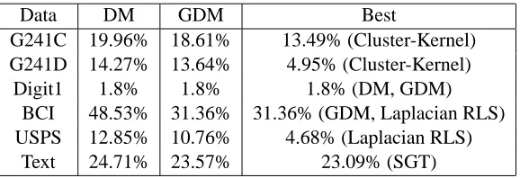
In this section we motivate the efficacy of the GDM approach with an empirical study of predic-tive accuracy in the semi-supervised setting on six benchmark data sets found in Chapelle et al. (2006). In the semi-supervised setting using the labeled as well as the unlabeled data for dimension reduction followed by fitting a regression model has often increased predictive accuracy. We used the benchmark data so we could compare the performance of DM and GDM to eleven algorithms (Chapelle et al., 2006, Table 21.11). The conclusion of our study is that GDM improves predictive accuracy over DM and that GDM is competitive with respect to the other algorithms.

For each data set twelve splits were generated with 100 samples labeled in each split. We applied DM and GDM to each of these sets to find DR directions. We projected the data (labeled and unlabeled) onto the DR directions and used a k-Nearest-Neighbor (kNN) classifier to classify the unlabeled data. The parameters of the DM, GDM, and number of neighbors were set using a validation set in each trial. The average classification error rate for the unlabeled data over the twelve splits are reported in Table 1. We also report in Table 1 the top performing algorithm for the data sets in Chapelle et al. (2006, Table 21.11). Laplacian RLS stands for Laplacian regularized least-squares, SGT stands for spectral graph transducer, Cluster-Kernel is an algorithm that uses two kernel functions, see (Chapelle et al., 2006, Chapter 11) for details.

A reasonable conclusion from Table 1 is that having label information improves the performance of diffusion operator with respect to prediction. In addition, dimension reduction using GDM fol-lowed by a simple classifier is competitive to other approaches. We suspect that integrating GDM with a penalized classification algorithm in the same spirit as Laplacian regularized least-squares can improve performance.

5. Graphical Models and Conditional Independence

One example of a statistical analysis where global inferences are desired or explanations with re-spect to the coordinates of the data is important is a graphical model over undirected graphs. In this setting it is of interest to understand how coordinates covary with respect to variation in response, as is provided by the GOP. Often of greater interest is to infer direct or conditional dependencies between two coordinates as a function of variation in the response. In this section we explore how this can be done using the GOP.

Data DM GDM Best

G241C 19.96% 18.61% 13.49% (Cluster-Kernel)

G241D 14.27% 13.64% 4.95% (Cluster-Kernel)

Digit1 1.8% 1.8% 1.8% (DM, GDM)

BCI 48.53% 31.36% 31.36% (GDM, Laplacian RLS)

USPS 12.85% 10.76% 4.68% (Laplacian RLS)

Text 24.71% 23.57% 23.09% (SGT)

Table 1: Error rates for DM and GDM over six data sets reported in Chapelle et al. (2006, Table 21.11). The column ’Best’ reports the error rate for the algorithm with the smallest error of the 13 applied to the data.

(Speed and Kiiveri, 1986; Lauritzen, 1996) was developed for multivariate Gaussian densities

p(x)∝exp

−1₂xTJx+hTx

,

where the covariance is J−1and the mean is µ=J−1h. The result of the theory is that the precision

matrix J, given by J=Σ−1

X , provides a measurement of conditional independence. The meaning of this dependence is highlighted by the partial correlation matrix RX where each element Ri j is a measure of dependence between variables i and j conditioned on all other variables S/i j and i₆= j

Ri j=

cov(Xi,Xj|S/i j)

p

var(Xi|S/i j)

q

var(Xj|S/i j)

.

The partial correlation matrix is typically computed from the precision matrix J

Ri j=−Ji j/

p

JiiJj j.

In the regression and classification framework inference of the conditional dependence between explanatory variables has limited information. Much more useful would be the conditional depen-dence of the explanatory variables conditioned on variation in the response variable. In Section 2 we stated that both the covariance of the inverse regression as well as the gradient outer product matrix provide estimates of the covariance of the explanatory variables conditioned on variation in the response variable. Given this observation, the inverses of these matrices

JX|Y =Ω_X−_|1_Y and JΓ=Γ−1,

provide evidence for the conditional dependence between explanatory variables conditioned on the response. We focus on the inverse of the gradient outer product matrix in this paper since it is of use for both linear and nonlinear functions.

the factors can be estimated independent of the response variable and in the sparse graphical model the response variable is considered as just another node, the same as the explanatory variables. Our approach and the sparse factor models approach both share an assumption of sparsity in the number of factors or directions. Sparse graphical model approaches assume sparsity of the partial correlation matrix.

Our proof of the convergence of the estimated conditional dependence matrix(Γˆ)−1_{to the} pop-ulation conditional dependence matrixΓ−1relies on the assumption that the gradient outer product matrix being low rank. This again highlights the difference between our modeling assumption of low rank versus sparsity of the conditional dependence matrix. Since we assume that bothΓand ˆΓ are singular and low rank we use pseudo-inverses in order to construct the dependence graph.

Proposition 13 LetΓ−1 be the pseudo-inverse ofΓ. Let the eigenvalues and eigenvectors of ˆΓbe

ˆ

λi and ˆvi respectively. If ε>0 is chosen so thatε=εn=o(1) andε−n1kΓˆ−Γk=o(1), then the

convergence

∑

ˆ

viˆλ−i 1vˆi n→∞ −→Γ−1

holds in probability.

Proof We have shown in Proposition 9 that_kΓˆ₋Γ_k=o(1). Denote the eigenvalues and eigenvec-tors ofΓasλiand virespectively. Then

|λˆi−λi|=O(kΓˆ−Γk) and kvˆi−vik=O(kΓˆ−Γk).

By the conditionε−_n1_kΓˆ₋Γ_k=o(1)the following holds ˆ

λi>ε=⇒λi>ε/2=⇒λi>0

implying_{i : ˆλi>ε} ⊂ {i :λi>0}in probability. On the other hand, denotingτ=min{λi:λi>0}, the conditionεn=o(1)implies

{i :λi>0}={i :λ≥τ} ⊂ {i : ˆλi≥τ/2} ⊂ {i : ˆλi>ε}

in probability. Hence we obtain

{i :λi>0}={i : ˆλi>ε}

in probability.

For each j_{∈ {}i :λi>0}we haveλj,ˆλj≥τ/2 in probability, so

|λˆ−j1−λ−j1| ≤ |λˆj−λj|/(2τ) n_→∞ −→0.

Thus we finally obtain

∑

ˆ

viˆλ−i 1vˆi n→∞

−→

∑

λi>0

viλ−i 1v T

5.1 Results on Simulated and Real Data

We first provide an intuition of the ideas behind our inference of graphical models using simple sim-ulated data. We then apply the method to study dependencies in gene expression in the development of prostate cancer.

5.1.1 SIMULATEDDATA

The following simple example clarifies the information contained in the covariance matrix as well as the gradient outer product matrix. Construct the following dependent explanatory variables from standard random normal variablesθ1, ...,θ5

iid

∼

N

X1=θ1,X2=θ1+θ2,X3=θ3+θ4,X4=θ4,X5=θ5−θ4, and the following response

Y =X1+ (X3+X5)/2+ε1, whereε1∼

N

We drew 100 observations(x_i1,x_i2,x_i3,x_i4,x_i5,yi)100i=1 from the above sampling design. From this data we estimate the covariance matrix of the marginals ˆΣX and the gradient outer product matrix

ˆ

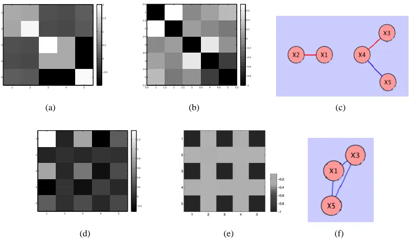
Γ. From ˆΣX, Figure 2(a), we see that X1and X2covary with each other and X3,X4,X5covary. The conditional independence matrix ˆRX, Figure 2(b), provides information on more direct relations between the coordinates as we see that X5 is independent of X3 given X4, X5 ⊥⊥X3|X4. The dependence relations are summarized in the graphical model in Figure 2(c). Taking the response variable into account, we find in the gradient outer product matrix, Figure 2(d), the variables X2and

X4are irrelevant while X1,X3,X5are relevant. The matrix ˆR_Γˆis shown in Figure 2(e) and implies that any pair of X1,X3,X5 are negatively dependent conditioned on the other and the response variable

Y . The graphical model is given in Figure 2(f).

5.1.2 GENESDRIVINGPROGRESSION OF PROSTATECANCER

A fundamental problem in cancer biology is to understand the molecular and genetic basis of the progression of a tumor from less serious states to more serious states. An example is the progression from a benign growth to malignant cancer. The key interest in this problem is to understand the genetic basis of cancer. A classic model for the genetic basis of cancer was proposed by Fearon and Vogelstein (1990) describing a series of genetic events that cause progression of colorectal cancer.

In Edelman et al. (2008) the inverse of the gradient outer product was used to infer the depen-dence between genes that drive tumor progression in prostate cancer and melanoma. In the case of melanoma the data consisted of genomewide expression data from normal, primary, and metastatic skin samples. Part of the analysis in this paper was inference of conditional dependence graphs or networks of genes that drive differential expression between stages of progression. The gradi-ent outer product matrix was used to infer detailed models of gene networks that may drive tumor progression.

1 2 3 4 5 1 2 3 4 5 −0.5 0 0.5 1 1.5 2 (a)

0.5 1 1.5 2 2.5 3 3.5 4 4.5 5 5.5 0.5 1 1.5 2 2.5 3 3.5 4 4.5 5 5.5 −1 −0.8 −0.6 −0.4 −0.2 0 0.2 0.4 0.6 (b) (c)

1 2 3 4 5 1 2 3 4 5 −0.2 0 0.2 0.4 0.6 0.8 1 1.2

(d) (e) (f)

Figure 2: (a) Covariance matrix ˆΣX; (b) Partial correlation matrix ˆRX; (c) Graphical model repre-sentation of partial correlation matrix; (d) Gradient outer product matrix ˆΓ; (e) Partial correlations ˆR_Γˆ with respect to ˆΓ; (f) Graphical model representation of ˆR_Γˆ.

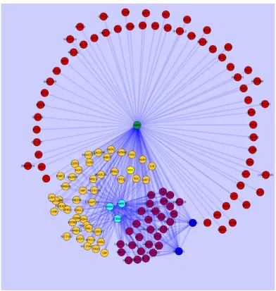
2008). For each sample the expression level of over 12,000 probes corresponding to genes were measured. We eliminated many of those probes with low variation across all samples resulting in a 4095 probes or variables. From this reduced data set we estimated the gradient outer product matrix, ˆΓ, and used the pseudo-inverse to compute the conditional independence matrix, ˆJ= (Γˆ)−1_. From the conditional independence matrix we computed the partial correlation matrix ˆR where

ˆ

Ri j =− ˆ Ji j

√_ˆ JiiJˆj j

for i₆= j and 0 otherwise. We again reduced the R matrix to obtain 139 nodes and

400 edges corresponding to the largest partial correlations and construct the graph seen in Figure 3.

Figure 3: Graphical model of genes relevant in tumors progressing from benign to malignant prostate tissue. The edges correspond to partial correlations.

6. Discussion

be-tween graphical models and dimension reduction intriguing and suggest that the manifold learning perspective holds potential in the analysis and inference of graphical models.

Acknowledgments

This work was partially supported by NSF grant DMS-0732260, NIH Systems Biology Center Grant, and NIH R01 CA123175-01A1. MM is grateful for partial support from NSF (DMS 0650413, IIS 0803293), ONR N00014-07-1-0625, the Sloan Foundation and Duke.

References

R.J. Adcock. A problem in least squares. The Analyst, 5:53–54, 1878.

M. Belkin and P. Niyogi. Laplacian Eigenmaps for Dimensionality Reduction and Data representa-tion. Neural Computation, 15(6):1373–1396, 2003.

M. Belkin and P. Niyogi. Semi-Supervised Learning on Riemannian Manifolds. Machine Learning, 56(1-3):209–239, 2004.

M. Belkin and P. Niyogi. Towards a theoretical foundation for Laplacian-based manifold methods. In Learning Theory, volume 3559 of Lecture Notes in Comput. Sci., pages 486–500. Springer, Berlin, 2005.

C. Carvalho, J. Lucas, Q. Wang, J. Chang, J. Nevins, and M. West. High-dimensional sparse fac-tor modelling - applications in gene expression genomics. Journal of the American Statistical

Association, 103(484):1438–1456, 2008.

O. Chapelle, B. Sch¨olkopf, and A. Zien, editors. Semi-Supervised Learning. MIT Press, Cambridge,

MA, 2006. URLhttp://www.kyb.tuebingen.mpg.de/ssl-book.

R.R. Coifman and S. Lafon. Diffusion maps. Applied and Computational Harmonic Analysis, 21 (1):5–30, 2006.

R.R. Coifman and M. Maggioni. Diffusion wavelets. Applied and Computational Harmonic

Anal-ysis, 21(1):53–94, 2006.

R.R. Coifman, S. Lafon, A.B. Lee, M. Maggioni, B. Nadler, F. Warner, and S.W. Zucker. Geomet-ric diffusions as a tool for harmonic analysis and structure definition of data: Diffusion maps.

Proceedings of the National Academy of Sciences, 102(21):7426–7431, 2005a.

R.R. Coifman, S. Lafon, A.B. Lee, M. Maggioni, B. Nadler, F. Warner, and S.W. Zucker. Geometric diffusions as a tool for harmonic analysis and structure definition of data: Multiscale methods.

Proceedings of the National Academy of Sciences, 102(21):7432–7437, 2005b.

R.D. Cook. Fisher lecture: Dimension reduction in regression. Statistical Science, 22(1):1–26, 2007.

R.D. Cook and S. Weisberg. Discussion of “Sliced inverse regression for dimension reduction”. J.

M. P. do Carmo. Riemannian Geometry. Birkh¨auser, Boston, MA, 1992.

D. Donoho and C. Grimes. Hessian eigenmaps: new locally linear embedding techniques for high-dimensional data. Proceedings of the National Academy of Sciences, 100:5591–5596, 2003.

N. Duan and K.C. Li. Slicing regression: a link-free regression method. Ann. Statist., 19(2):505– 530, 1991.

E.J. Edelman, J. Guinney, J-T. Chi, P.G. Febbo, and S. Mukherjee. Modeling cancer progression via pathway dependencies. PLoS Comput. Biol., 4(2):e28, 2008.

F.Y. Edgeworth. On the reduction of observations. Philosophical Magazine, pages 135–141, 1884.

J. Fan and I. Gijbels. Local Polynomial Modelling and its Applications. Chapman and Hall, London, 1996.

E.R. Fearon and B. Vogelstein. A genetic model for colorectal tumorigenesis. Cell, 61:759–767, 1990.

R.A. Fisher. On the mathematical foundations of theoretical statistics. Philosophical Transactions

of the Royal Statistical Society A, 222:309–368, 1922.

K. Fukumizu, F.R. Bach, and M.I. Jordan. Dimensionality reduction in supervised learning with reproducing kernel Hilbert spaces. Journal of Machine Learning Research, 5:73–99, 2005.

E. Gin´e and V. Koltchinskii. Empirical graph Laplacian approximation of Laplace-Beltrami oper-ators: large sample results. In High dimensional probability, volume 51 of IMS Lecture Notes

Monogr. Ser., pages 238–259. Inst. Math. Statist., Beachwood, OH, 2006.

G.H. Golub and C.F. Va Loan. Matrix Computations. The Johns Hopkins University Press; 3rd edition, 1996.

T. Hastie and R. Tibshirani. Discriminant analysis by Gaussian mixtures. J. Roy.Statist. Soc. Ser. B, 58(1):155–176, 1996.

C-H. Hsiang, T. Tunoda, Y.E. Whang, D.R. Tyson, and D.K. Ornstein. The impact of altered annexin i protein levels on apoptosis and signal transduction pathways in prostate cancer cells.

The Prostate, 66(13):1413–1424, 2004.

Z. Jiang, B.A. Woda BA, C.L. Wu, and X.J. Yang. Discovery and clinical application of a novel prostate cancer marker: alpha-methylacyl CoA racemase (P504S). Am. J. Clin. Pathol, 122(2): 275–8941, 2004.

G . Kramer, G. Steiner, D. Fodinger, E. Fiebiger, C. Rappersberger, S. Binder, J. Hofbauer, and M. Marberger. High expression of a CD38-like molecule in normal prostatic epithelium and its differential loss in benign and malignant disease. The Journal of Urology, 154(5):1636–1641, 1995.

K.C. Li. Sliced inverse regression for dimension reduction. J. Amer. Statist. Assoc., 86:316–342, 1991.

K.C. Li. On principal Hessian directions for data visualization and dimension reduction: another application of Stein’s lemma. Ann. Statist., 97:1025–1039, 1992.

N. Meinshausen and P. Buhlmann. High-dimensional graphs and variable selection with the Lasso.

Annals of Statistics, 34(2):1436–1462, 2006.

S. Mukherjee and Q. Wu. Estimation of gradients and coordinate covariation in classification. J.

Mach. Learn. Res., 7:2481–2514, 2006.

S. Mukherjee and DX. Zhou. Learning coordinate covariances via gradients. J. Mach. Learn. Res., 7:519–549, 2006.

S. Mukherjee, D-X. Zhou, and Q. Wu. Learning gradients and feature selection on manifolds.

Bernoulli, 16(1):181–207, 2010.

S. Roweis and L. Saul. Nonlinear dimensionality reduction by locally linear embedding. Science, 290:2323–2326, 2000.

T. Speed and H. Kiiveri. Gaussian Markov distributions over finite graphs. Ann. Statist., 14:138– 150, 1986.

M. Sugiyama. Dimensionality reduction of multimodal labeled data by local fisher discriminant analysis. J. Mach. Learn. Res., 8:1027–1061, 2007.

A. Szlam, M. Maggioni, and R. R. Coifman. Regularization on graphs with function-adapted diffu-sion process. J. Mach. Learn. Res., 9:1711–1739, 2008.

M. Szummer and T. Jaakkola. Partially labeled classification with markov random walks. In T. Di-etterich, S. Becker, and Z. Ghahramani, editors, Advances in Neural Information Processing

Systems, volume 14, pages 945–952, 2001.

J. Tenenbaum, V. de Silva, and J. Langford. A global geometric framework for nonlinear dimen-sionality reduction. Science, 290:2319–2323, 2000.

S.A. Tomlins, R. Mehra, D.R. Rhodes, X. Cao, L. Wang, S.M. Dhanasekaran, S. Kalyana-Sundaram, J.T. Wei, M.A. Rubin, K.J. Pienta, R.B. Shah, and A.M. Chinnaiyan. Integrative molecular concept modeling of prostate cancer progression. Nature Genetics, 39(1):41–51, 2007.

G. Wahba. Splines Models for Observational Data. Series in Applied Mathematics, Vol. 59, SIAM, Philadelphia, 1990.

Q. Wu, F. Liang, and S. Mukherjee. Regularized sliced inverse regression for kernel models. Tech-nical Report 07-25, ISDS, Duke Univ., 2007.

Y. Xia, H. Tong, W. Li, and L-X. Zhu. An adaptive estimation of dimension reduction space. J.

L. Zwald and G. Blanchard. On the convergence of eigenspaces in kernel principal component analysi s. In Y. Weiss, B. Sch¨olkopf, and J. Platt, editors, Advances in Neural Information