Obtaining the Knowledge of a Server Performance from Non-Intrusively
Measurable Metrics
Satoru Ohta
*Department of Information Systems Engineering, Toyama Prefectural University, Imizu, Japan.
Received 15 January 2016; received in revised form 13 March 2016; accepted 16 March 2016
Abstract
Most network services are provided by server computers. To provide these services with good quality, the server
performance must be managed adequately. For the server management, the performance information is commonly
obtained from the operating system (OS) and hardware of the managed computer. However, this method has a
disadvantage. If the performance is degraded by excessive load or hardware faults, it becomes difficult to collect and
transmit information. Thus, it is necessary to obtain the information without interfering with the server’s OS and
hardware. This paper investigates a technique that utilizes non-intrusively measureable metrics that are obtained
through passive traffic monitoring and electric currents monitored by the sensors attached to the power supply.
However, these metrics do not directly represent the performance experienced by users. Hence, it is necessary to
discover the complicated function that maps the metrics to the true performance information. To discover this
function from the measured samples, a machine learning technique based on a decision tree is examined. The
technique is important because it is applicable to the power management of server clusters and the immigration
control of virtual servers.
Keywords: machine learning, network servers, performance management, traffic measurement
1.
Introduction
Most network services are provided by server computers. To provide these services with good quality, the server
performance must be managed adequately. The providers of services must monitor the server performance. If they find
anomalies or degradation of the server performance, they must take appropriate actions to keep service quality. The
performance information is also essential for the various traffic and resource control, which includes, for example, load
balancing among the server computers [1] and the power saving of a server cluster [2-3].
Clearly, the server performance is related to the utilization of resources. If the capacity of a resource is exhausted, the
performance will degrade. Thus, the utilization of a resource can be used as the metric for performance. Actually, the
utilizations of resources such as CPU, network interfaces, disks, etc., have been used as metrics for various types of server
management. For example, the power management technique reported in [4] uses the CPU and disk utilizations to decide which
computers in a cluster should be turned on or off. Similarly, the CPU utilization, the I/O usage and the network usage are used
in [5] to manage virtual machines constructed on a server computer.
Although the resource utilization provides some information on performance, it is not strictly adequate to monitor the
resource utilization for understanding the performance experienced by users. A server computer consists of various resources.
However, it is difficult to monitor the utilizations for all of these physical parts and network buffers. Moreover, the performance
metric, such as response time, is not directly represented by the resource utilizations. That is, the performance is usually
represented by a complicated function of the resource utilizations.
Another issue is that the resource utilization data is gathered trough the server computer resources, which are the objectives
of the management. This means, if some resources do not operate correctly because of overload or failure, the resource
utilization data may not be obtained. The operating system (OS) of a server machine provides some information of physical
resource usages including CPU, disk, and network interfaces. However, the OS must always work correctly to gather these
utilization metrics successfully. If the CPU (or memory, bus, network, or other resources) is overloaded by excessively many
service requests from users, the performance of the OS itself will degrade. For that case, it becomes difficult for the management
system to obtain the utilization data through the OS. The only method that avoids this problem is to collect information without
interfering any resources of the server computer.
To find the server performance from the non-intrusively measured metrics, it is necessary to clarify the relationship
between them. It is difficult to theoretically analyze the function that maps the metrics to the performance. Therefore, it is
necessary to build the function from the measured samples of the metrics and performance. The machine learning technique is
a powerful tool to obtain this function.
This paper investigates a technique that utilizes non-intrusively measureable metrics. These metrics are passively
measured traffic metrics and the electric currents monitored by the sensors attached to the power supply lines. Unfortunately,
these metrics do not directly represent the performance experienced by users. Hence, it is necessary to discover t. To discover he
complicated function that maps the metrics to the performance, a machine learning technique based on a decision tree is
examined. The feasibility and effectiveness of the metrics and the machine learning technique are assessed through experiments.
In the experiments, the World Wide Web is assumed as the service provided by the server. However, it is considered the
presented technique will be effective for other network services as well. The technique is important because of applications
including the load balancing in a server cluster, the power management of a server cluster and the immigration control of virtual
servers.
The rest of the paper is organized as follows. Section 2 explores the relationship between resource utilization and server
performance. The advantage of non-intrusive measurement is explained in Section 3. As non-intrusively measurable metrics,
traffic attributes are examined in Section 4 while electric currents are examined in Section 5. In Section 6, the applications of
this study are overviewed. Finally, Section 7 concludes the paper.
2.
Resource Utilization and Performance
A server computer consists of various resources. These include physical parts such as CPU, memory, bus, disks and
network interfaces. Additionally, the performance of network services depends on various buffers including
receipt/transmission buffers and the request accept queue for the TCP-based services. These buffers are also considered as
server resources and related to the performance. Other network related parameters, for example, the maximum number of
available TCP sockets, may affect the performance. It depends on the provided service content which resource is first exhausted
and network buffers. Additionally, the utilizations of some physical resources such as CPU or disk are available through the OS,
while those of the other resources are invisible to the management system.
The relationship between the resource utilizations and the server performance is not simple. Moreover, it is difficult to
discover the performance degradation by monitoring only a few resource utilizations. This characteristic is shown through the
experiment, which was executed on two Linux PCs connected by 1 Gb/s Ethernet. The Ethernet connection was established by
a cross-over cable, which directly connects these PCs. The PCs have the Celeron 3.06 GHz CPU, 512MB RAM, and 80GB disk.
A WWW server (Apache) runs on one PC, while a client program runs on the other PC. The client program is httperf [6],
which requests page data to the server with a specified rate as well as outputs the server performance. From the output of the
httperf program, the satisfaction of the performance criteria is checked. The output of the httperf program was also used
to estimate the bit rate from the server to the client. On the server PC, the CPU utilization was measured with using the top
command. The page data placed on the server PC consists of multiple file sets. The employed file sets are summarized in
Table 1.
Table 1 File sets served by the server PC
Set #1 Heavy load PHP script
Set #2 Medium load PHP script
Set #3 Light load PHP script
Sets #4#13
100 html files, size of each file: 300 B, 1 KB, 10 KB, 30 KB, 60 KB, 100 KB, 300 KB, 1 MB, 10 MB, 30 MB
Among the file sets, the sets #1, #2 and #3 are basically the same PHP script. This script outputs an html file that includes
a sequence of random m words as its body content. A word is constructed by n characters selected from 30 letters, which are
lowercase alphabets, a space, a colon, a comma and a period. The words are given as constants. Meanwhile, the word sequence
is generated for each request by executing the PHP mt_random() function [7] m times to randomly select words. Therefore,
for a larger value of m, the computational load becomes heavier because the number of repetition grows greater. Thus, m and n
were set as follows to generate heavy, medium and light loads.
Set #1: m = 500,000, n = 2
Set #2: m = 100,000, n = 10
Set #3: m = 10,000, n = 100
As a metric of the performance experienced by a user, the connection time, which is shown in the httperf output. Fig. 1
shows the connection time against the CPU utilization for the heavy load PHP file (set #1), the 10 KB files (set #6) and the 1 MB
files (set #11). The figure shows that the performance degrades at a particular CPU utilization. More importantly, the CPU
utilization where the performance degrades is quite different depending on the file set. For the set of 1 MB files, the connection
time increases at a very small CPU utilization. Clearly, for this file set, the computational capacity of the CPU is sufficient and
thus the performance is limited by the bottleneck resource other than the CPU. By contrast, for the PHP script, the performance
degrades when the CPU utilization becomes very close to 100 %. This suggests that the performance is mostly limited by the
CPU. The result concludes that it is impossible to find the performance degradation by monitoring only the CPU utilization.
Even if we set some threshold value for the CPU utilization to detect the degradation, the threshold value will be too small for
the PHP script or too large for the 1 MB files. That is, the appropriate threshold value cannot be determined so as to be effective
0.0 10.0 20.0 30.0 40.0 50.0 60.0
1.0 10.0 100.0
Conn
ect
ion
Es
tab
lish
men
t
Time (
ms)
CPU Utilization (%)
Heavy Load PHP 10 KB Files 1 MB Files
Fig. 1 Connection time versus the CPU utilization
Fig. 2 plots the connection time against the bit rate for the heavy load PHP file, the 10 KB files and the 1 MB files. The
figure shows that the connection time quickly increases at a particular bit rate. The bit rate where the performance degrades is
very different depending on the file set similarly to the CPU utilization case. For the PHP script, the connection time increases
at a low bit rate. This is because the transmitted data size is small but the CPU consumption is heavy. Thus, the bottleneck is the
CPU for this file set and the network resource is abundant. Meanwhile, for the 1 MB files, the connection time increases at a
high bit rate. For this file set, the performance is limited by the capacity of the network interface. Thus, the degradation is not
detected by monitoring only the bit rate because the threshold for determining the degradation cannot be chosen so as to be valid
for every file set.
0.0 10.0 20.0 30.0 40.0 50.0 60.0
1.0E+03 1.0E+04 1.0E+05 1.0E+06
Conn
ect
ion
Es
tab
lish
men
t
Time (
ms)
Bit Rate (b/s) Heavy Load PHP 10KB Files
1 MB Files
Fig. 2 Connection time versus the bit rate
The above results suggest that it is inadequate to judge the performance by monitoring only one utilization parameter. Then,
what happens if we use two utilization parameters? Fig. 3 shows the relationship between two resource utilizations, where the
server performance degrades. The performance degradation is judged by the increase of the connection establishment time. As
shown in Figs. 1 and 2, the connection time is less than 1 ms for light load. Meanwhile, it quickly increases to some ten
milliseconds when the resource utilization exceeds a certain value. Obviously, this region of resource utilization indicates the
degradation of server performance. Consequently, some ten milliseconds of the connection time can be considered as an
evidence of degradation. With considering this characteristic, the criterion for the degradation is that the connection time
points for the PHP scripts, the points for the 100 B to 1 MB files, and the points for the file sets of 10 and 30 MB. The plotted
points are completely separated and are difficult to be connected. The figure clearly implies that these distinct groups are
brought by the different in performance limitation mechanisms.
0.1 1.0 10.0 100.0
1.0E+03 1.0E+04 1.0E+05 1.0E+06
CPU
U
til
iza
ti
on
(%)
Bit Rate (b/s) File Sets #1-#3 File Sets #4-#11 File Sets #12 & #13
Fig. 3 Bit rate and CPU utilization where the performance degrades
The difference in the performance limitation is explained as follows. Since the PHP scripts offer heavy computations for
the server computer, the performance is limited by the computational capacity of the CPU. For the 100B to 1 MB file sets, the
computational load is not heavy as for the PHP script case. Additionally, the page data will be cached to the main memory of the
server computer since the file size is small. Thus, the disk I/O speed does not affect the performance for these file sets. Therefore,
it is rational to consider that the network interface capacity dominantly determines the performance. By contrast, for the file sets
of 10 and 30 MB, the page data is too large to be cached for the main memory. Thus, the page data are read out from the disk for
these file sets to reply each page request. This means that the disk I/O speed limits the performance. This difference in the
performance bottlenecks brings the three separated plot groups shown in Fig. 3.
If the CPU utilization and the bit rate are on the upper-right side of the curve, the connection time gets greater than the
criterion. Thus, to detect the performance degradation from the CPU utilization and the bit rate, the function that represents the
curves must be found. It is not easy to analytically obtain the function that represents each curve. Obviously, additional metrics
are necessary to find degradation. Otherwise, it is impossible to distinguish which of three groups shown in Fig. 3 should be
adequate for the degradation detection. Thus, the border of performance degradation is expressed as a function of three or more
metrics. The performance is related to many computer resources, including network buffers, are related to the performance.
Therefore, the difference of the relevant resources may require more metrics. This implies that the problem of detecting the
performance degradation is to find the complicated function of multiple metrics. Since the theoretical analysis is difficult, the
function must be determined from the measured samples. To attain this purpose, the machine learning technique is a powerful
tool.
3.
Non-Intrusive Measurement
The resource utilizations of a computer are often measured by the OS and provided to a user program. For example, the
utilizations of the resources such as the CPU, the network interface and the disk I/O are obtained through the pseudo files under
the /proc directory on the Linux OS. However, this information is not very reliable when a failure occurs on the managed
resources. For example, if the OS hangs, it becomes impossible to obtain these utilization metrics. Needless to say, if a failure
the resource capacity, the performance of the OS and the management software will be degraded. This also makes it difficult to
extract the resource utilization information.
The information on the server performance is particularly important when the performance approaches to degradation by
excessively heavy load. The information is also required to see the operating status of the resources when a failure is presumed.
However, in these situations, where the utilization information is particularly needed, the OS may not provide the resource
utilizations successfully.
To find the server performance under the excessively heavy load or resource failures, the information that reflects the
performance must be obtained completely without using the resource of the managed computer. In other words, the performance
should be estimated in the “out-band” or non-intrusive method; the performance data must be separated from the computer
resource and the user data associated with the service. This non-intrusive method is also advantageous because it does not rely
on a particular hardware architecture or OS of the managed server computer. Thus, the method is universally applicable to any
hardware or OS.
As a non-intrusive approach, this study examines two types of metrics that reflect the performance information. One is the
network traffic metrics obtained from the captured packets while the other is the electric currents monitored through current
sensors attached to the power supply lines of the computer. The following sections explore the details of these metrics. It is also
described how the machine learning technique is applied to find the function that maps the metrics to the performance.
4.
Traffic Attributes and Performance
This section presents how the server performance degradation is detected through traffic measurement. First, the
informative traffic metrics are identified. Then, it will be shown how the deterioration is judged from these metrics with using a
machine learning technique. The effectiveness of this approach is assessed through experiment.
4.1. Overview
The change of the server performance will be reflected on the network traffic. The traffic can be passively monitored by
capturing packets on a machine that is separate from the managed server computer. Thus, the information is non-intrusively
extracted without using any resource of the managed server computer.
4.2. Metrics
The performance information is included in several attributes of the monitored traffic. As the attributes that are informative
and easy to be obtained, this study examines the bit rate, the packet rate, the connection rate, the number of flows and the TCP
SYN loss rate. These metrics are obtained from the packets captured during a constant measurement period. The definition,
necessity and measurement method of these attributes are detailed as follows.
4.2.1 Bit rate
The bit rate is the number of the bits transmitted in a unit time. Since the bit rate on a transmission link cannot be higher
than its capacity, the bit rate is clearly informative for the link utilization and the performance. If the bit rate approaches to the
capacity of the transmission link, many packets will be queued to the output buffer. Since this situation will cause large queuing
delay or packet loss, the performance will be degraded. Obviously for this degradation case, the bit rate will be an essential
The bit rate is easily measured by summing the bit length of the arrived packets and then dividing the total bit number with
the measurement period.
4.2.2 Packet rate
The packet rate in the number of the packets transmitted in a unit time. A network interface must execute the process
associated with each packet. Since the capacity of processing packets is limited, there exists an upper limit for the packet rate.
Because of this, the throughput of a network interface often decreases for shorter packets. Thus, for the services that issue many
short packets, the packet rate may determine the performance. Therefore, the packet rate will be necessary as performance
information.
The packet rate is obtained by counting the arrived packets and then dividing the total packet number with the
measurement period.
4.2.3 Connection rate
The connection rate is the number of established TCP connections during a unit time. When a TCP connection is set up or
cleared, some process associated with the connection is invoked. Since this process consumes resources, an excessively high
connection rate may degrade the performance.
The establishment of a TCP connection is found by a SYN ACK message. Thus, the connection rate is estimated by the
ratio of the SYN ACK message number and the measurement period. The SYN ACK messages are found by filtering the arrived
packets with the SYN and ACK flags in the TCP header.
4.2.4 Number of flows
A flow is the set of packets that have the same flow identifier. A flow identifier is a set of fields in the packet header. This
study defines the flow identifier by a five tuple of the protocol, source address, destination address, source port, and destination
port as often found in literature [8-9]. With this flow identifier definition, it is obvious that a flow corresponds to an open socket
or a connection for the TCP communication. The number of flows is how many flows exist during a unit time.
The significance of the flow number is understood by the following example. Suppose that a TCP-based network service is
provided on a network interface. Then, consider the following two cases, which are different in the flow number. That is, there
are only 10 flows for one case while there are 1000 flows for the other case. Assume that the bit rate of the traffic is 900 Mb/s for
both cases. Then, the quality of the service is obviously very different between the cases. For the former case, the average bit
rate of a flow is 90 Mb/s. This bit rate suggests a very good service quality. By contrast, the average bit rate of a flow is as small
as 0.9 Mb/s for the latter case. This may cause serious performance degradation, such as an unacceptable increase of the
download time. Thus, the number of flow may reveal the performance degradation, which cannot be found by the total bit rate
or packet rate.
The number of flows is counted by the methods reported in [8, 10-11]. These methods are basically based on the linear
counting algorithm [12], which counts the number of distinct items in a large database. That is, the problem is to count the
distinct flow identifiers among those of the packets arrived during a unit time. This study counts the flows with using the method
of [11]. In the experiment described later, the flow is counted every 1 second and then the flow number is averaged over the
4.2.5 TCP SYN loss rate
The TCP SYN loss rate is the ratio of the TCP SYN messages that are not responded with the SYN ACK messages.
Specifically, let NS and NA denote the numbers of TCP SYN and SYN ACK messages seen in the measurement period. Then, the
TCP SYN loss rate R is,
S A A N N R N (1)
It is reported [13] that the delay in the socket accept queue grows rapidly when a heavy load is offered to the Apache
WWW server. If the queue length increases, the TCP SYN messages will be overflown from the buffer with a high probability.
By the loss of a TCP SYN message, the client must retransmit the message after timeout. This retransmission greatly increases
the response time [14]. Thus, a large value of the TCP SYN loss rate means that many clients experience the degraded response
time. Thus, the TCP SYN loss rate is a relevant metric for the TCP-based server performance [1].
The TCP SYN loss rate is obtained by counting the TCP SYN and SYN ACK messages from the packets captured during
the measurement time. The TCP SYN and SYN ACK messages are easily extracted from other packets by checking the SYN
and ACK flags shown in the TCP header.
4.3. Finding Performance Degradation
The objective is to find the server performance degradation from the traffic metrics described above. Let x1, x2, x3, x4 and
x5 denote the bit rate, the packet rate, the connection rate, the number of flows and the TCP SYN loss rate, respectively.
Additionally, let x denote the vector (x1, x2, x3, x4, x5). Then, the problem is to discover the function f(x) such as,
good. ly sufficient not is e performanc the if NG, good. ly sufficient is e performanc the if OK, ) (x f (2)
It is difficult to determine the function f(x) analytically because the relationship between the performance and the traffic
metric x is not theoretically clear. Meanwhile, it is easy to build the function f(x) from samples with using the machine learning
technique.
The machine learning technique is described as follows. Suppose that a system state falls into one of the n classes s1, …, sn.
We can observe m attributes a1, …, am, which provide some information about the unknown current state class. The value of
each attribute is determined according to some probability distribution, which depends on the current class. Then, the purpose of
machine learning is to build a classifier that estimates the unknown current class from the measured attribute values. Assume
that we have training data, which includes the vectors of the actual class as well as the attribute values measured under that class.
For this situation, a machine learning algorithm exists that builds a classifier from the training data.
The above framework of machine learning is applied to this study by considering the traffic metrics x as the attributes and
the OK/NG as the classes. By applying the machine learning technique, the function f(x) is algorithmically obtained from the
measured samples. Although the form of the function varies according to the changes of the machine specification, the machine
setting or the service contents, the machine learning technique can easily adapt to the change by re-learning.
Known classifier models include Bayesian networks, decision trees, artificial neural networks, and support vector machine,
etc. Among these approaches, this study focuses on the decision tree. The decision tree classifier has been well studied and is
known to be reliable. As [15] points out, an advantage of the decision-tree-based method is its very low computational cost of
querying the trained classifier. This advantage is very important for real time performance management of servers. The method
advantages, the decision tree approach is used for various studies on system management [2, 16-19]. Thus, the approach is
considered sufficiently reliable. As a program for generating the decision tree classifier, c4.5 [20] is employed.
A decision tree is a rooted tree representing a sequential decision process in which attribute values are successively tested
to infer an unknown state. Fig. 4 shows an example of a decision tree. The inference process starts at its root and proceeds to a
leaf. An attribute is assigned to each internal node, while each leaf is labeled with the most likely state. When the process
reaches an internal node, the attribute assigned to the node is tested to decide which child node the process should proceed to.
When the process reaches a leaf, the leaf label is considered to be the current state class. The structure of the tree, the attributes
assigned to internal nodes, and the classes assigned to leaves are decided by a tree construction algorithm from the training data.
The c4.5 program builds a reliable decision tree classifier by using an algorithm based on the information theory.
a1
a2
a3
a1 a1
s1
s1 s1
s2
s3 s3
0
2
a a21
5
1
a a15
3
1
a a18
3
1
a a18
0
3
a a31
Root
a1, a2, a3: Attributes Leaf
S1, S2, S3: State Classes
Fig. 4 Decision tree example
4.4. Evaluation
To confirm the effectiveness of the above concept, an experiment was performed on the configuration shown in Fig. 5. The
system consists of 3 Linux PCs, PC1, PC2, and PC3. In the configuration of Fig. 5, each 1000Base-T Ethernet connection was
established by a cross-over cable, which directly connects two PCs. The PCs have the Celeron 3.06 GHz CPU, 512MB RAM,
and 80GB disk. On PC1, the apache web server runs. As a web client, httperf, a web benchmark software, was executed on
PC3. The class was determined by the output of the httperf. Two Ethernet interfaces were attached to PC2; one interface is
connected to PC1 while the other is connected to PC3. Different network addresses were assigned to these interfaces. This
means that PC2 plays a role of a router. The traffic metrics were measured on PC2. To obtain the traffic metrics, a C language
program was developed with using the pcap library [21], which provides the functions to capture the packets on a network
interface. With these traffic metrics and the class, the training data and test data were constructed. The program captures the
packets on the interface connected to PC1, and extracts the traffic metrics. The throughput of PC2 is sufficiently large as a router,
and the load generated by the traffic measurement program is low. Thus, the insertion of PC2 does not affect the performance of
a service provided between PC1 and PC3.
Apache Traffic Metrics Request Page Data Request Page Data httperf PC1 PC2 PC3 1000Base-T Ethernet (Cross-Over Cable)
To determine the performance class, the criteria for sufficiently good performance is necessary. Thus, server performance
is considered to be sufficiently good if both of the following two conditions are satisfied from the viewpoint of the WWW
application:
- The average time of the TCP connection establishment is less than 0.1 s.
- The average bit rate achieved on the application layer from the server to a client is greater than 10 MB/s.
These criteria are determined because of the following reasons. If the first condition is satisfied, the connection will be
established much faster than the time required by a user to accept the Web page response [22]. The satisfaction of the second
condition means that the bit rate is sufficiently large to perform, for example, movie streaming with DVD quality. Thus, it is
considered that the conditions are rational as performance criteria to serve a Web page that includes a movie.
The satisfaction of the above conditions is determined by the output of httperf. The output includes the average time of
the TCP connection establishment. Thus, the first condition can be examined directly from its output. The output also shows the
average data transfer time. Thus, the bit rate of the application layer is easily calculated by the ratio of the page data size and the
download time. This bit rate is used to test whether the second condition is satisfied or not.
As the web contents, the file sets shown in Table 1 were placed on PC3. An instance of the training and test data was
obtained as follows. The request for the page data of a file set is generated at a specified rate by httperf for about 5 minutes.
The class is obtained by the result of this 5 minutes measurement. Simultaneously, the traffic metrics are repeatedly measured
with the period of 1 minute by the traffic measurement program. Among the measured traffic metric sets, two sets recorded in a
steady state are selected for the training or test data instance. Thus, two training or test data instances were generated by the 5
minute httperf execution.
The request rate for each data instance was determined as follows. First, the maximum request rate that satisfies the
performance criteria was obtained for each file set by deciding the class for different request rates. Let RM denote this maximum
rate. Then, a data instance was taken for the request rate Ri (0i10) defined as,
M
i iR
R (0.750.05) (3)
The training data consists of the instances taken for file sets #1, #3, #5, #7, #9, #11 and #13 while the test data consists of
the instances taken for file sets #2, #4, #6, #8, #10, and #12. Thus, the file sets used for the test data were different from those
used for the training data. This setting will be helpful to confirm the generalization effect of the machine learning approach.
The above procedure produces 140 training data instances and 120 test data instances. The training data was inputted to the
c4.5 program, which built the decision tree. Then, the test data was fed to the decision tree. The class inferred by the decision
tree was compared with the true class. Then, the number of the incorrect inferences was counted. This testing process was also
executed by the c4.5 program.
The result of the class inference is shown in Table 2. As the table shows, the total number of errors for the file sets #2, #4,
#6, #8, #10, and #12 was 3 among 120 test data instances. Thus, the error rate is as small as 2.5 %. This concludes that the
decision classifier successfully inferred the performance class even though the contents used in the test data are different from
those used in the training data. The result also confirms that the traffic metrics are very informative to determine the server
Table 2 Inference result by the traffic metrics Inferred Class
OK NG
True Class
OK 66 0
NG 3 51
Among three error cases observed in the above result, two cases occurred for file set #10 (300KB files) and one case
occurred for file set #12 (10MB files). For the file set #10, the inferred class was incorrect when the request rate Riwas equal to
RM. The rate RM stands on the border between the classes OK and NG. Thus, it is easily understood that the decision for the rates
close to RM is difficult and may cause incorrect results. Meanwhile, the rate Ri was 1.15 RM when the error occurred for the file
set #12. The reason for this error is presently inconclusive.
5.
Electric Currents
This section explores how to detect performance degradation through electric currents. The section first presents how the
electric currents to CPU and hard disk drive are measured. Then, the relationship between the measured currents and resource
utilizations is clarified by experimental results. The accuracy of the degradation detection that uses electric currents is also
evaluated through experiments.
5.1. Overview
The change of the resource utilization is reflected on the electric currents provided by the power supply. If heavy
computation is executed on a computer, more electric current is sent to its CPU. By employing this characteristic, it becomes
possible to estimate the computational load on the CPU. Similarly, if hard disk access increases, the power provided to the disk
also increases. Thus, the degree of hard disk access can be estimated by monitoring the electric current. These current-based
estimation methods of the resources are very advantageous because they can be executed non-intrusively, completely without
touching the physical and logical resources of the managed computer. By adding the electric current information to the traffic
metric, it is expected that the accuracy of inferring the performance class will improve.
5.2. Method
This study examines the feasibility of estimating the resource utilization and the performance class from the electric
currents through experiments. The experiment was performed on the configuration shown in Fig. 6. As shown in the figure, the
configuration is basically identical to that shown in Fig. 5. The employed machines are the same as those used in Fig. 5. The
only difference is that the current sensors are attached to PC1, and the sensor output is recorded on PC2 via the amplifier and the
analog to digital conversion on the microcomputer.
Apache Traffic Metrics
Request
Page Data
Request
Page Data httperf
PC1 PC2
PC3
1000Base-T Ethernet
Current Sensor
Amplifier Microcomputer
USB
The electric currents were measured by two current sensors attached to PC1. The employed sensor is based on the Hall
device and can be attached to the power supply lines. One of the sensors is attached to the ATX-12V lines, which is connected
to the motherboard. As specified in the PC motherboard specification [23], the ATX-12V lines are connected to the processor
voltage regulator. Therefore, the current on these lines is sent to the CPU and thus expected to be informative for the
computational load. Meanwhile, the other sensor is attached to the +5V line for the SATA hard disk. This provides information
on the hard disk access. These monitored currents are termed the "CPU current" and the "HD current", respectively. Fig. 7
shows the sensor attached to the +5V line to the hard disk.
Fig. 7 Current sensor attached to the power supply line of the hard disk
Since the sensor output is not very large, the output is first enlarged by 40 times with an amplifier. Since the sensitivity of
the sensor is 20 mV/A, the amplifier output has the sensitivity of 0.8 V/A. The amplifier output is sampled and digitized by the
Arduino microcomputer [24]. The sampling interval is 10 milliseconds. The microcomputer also averages 100 sampled
amplifier outputs and sends the result to PC2 every 1 second through the USB cable. Fig. 8 shows the employed amplifier and
the microcomputer. On PC2, each current data is further averaged over 60 received values.
Fig. 8 Amplifier and microcomputer to process the sensor output
5.3. Evaluation
First, it was examined whether the CPU and HD currents are effective to evaluate the CPU and disk utilizations or not. The
program can generate the load with a specified CPU utilization. While the program ran on PC1 with varying the CPU utilization,
the CPU current monitored by the sensor was recorded. For each value of the CPU utilization, the current was measured for 60
seconds, and then the data was averaged. Fig. 9 shows the result. In the figure, the x-axis is the CPU utilization given to the
lookbusy program while the y-axis is the average CPU current observed by the sensor. The figure shows that the current
linearly increases for the increase of the CPU utilization. From the figure, it is obvious that the CPU utilization is easily
estimated by the CPU current without touching the OS or any other resource of the monitored computer.
0.0 0.5 1.0 1.5 2.0 2.5 3.0 3.5 4.0
0 20 40 60 80 100
CPU
Cur
ren
t
(A)
CPU Utilization (%)
Fig. 9 Relationship between the CPU utilization and the CPU current
Next, the estimation of the hard disk load by the HD current was assessed. This was performed by offering various hard
disk loads on the PC1 while measuring the HD current. The load was generated by the stress program [26]. By changing the
read/write byte volume given to the program, different loads were generated on the monitored PC. The actual disk load was
measured by the vmstat command. Among the outputs of the vmstat command, the input and output data bytes of the block
device (i.e., disk) was used as the disk load metric. The measurement period for the HD current was 60 seconds for each load
condition. Simultaneously, the output of vmstat was recorded to obtain the total byte volume during the 60 seconds.
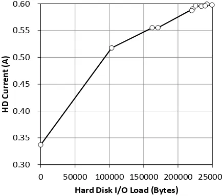
Fig. 10 shows the relationship of the load and the HD current. The HD current monotonously increases for the increase of
the hard disk load. It is observed that the current tends to saturate for larger loads. This may become a drawback to estimate
heavier loads exactly. Nevertheless, it is obvious that the HD current is useful to estimate the hard disk load to a certain extent.
0.30 0.35 0.40 0.45 0.50 0.55 0.60
0 50000 100000 150000 200000 250000
HD
Cur
ren
t
(A)
Hard Disk I/O Load (Bytes)
Finally, the effectiveness of the current information in inferring performance class was examined through an experiment.
For the class inference, the machine learning based on the decision tree was used again. While the traffic metrics data was
gathered for the traffic-based inference experiment, the CPU and HD currents of the PC1 were simultaneously recorded with the
configuration of Fig. 6. The attributes of a data instance are the CPU and HD currents measured during the 60 seconds period,
where the server is in a steady state. Among the 5 minute page request period, two steady state periods were selected as in the
traffic-based inference case, and thus two data instances were obtained. The CPU and HD current data was sampled with 10ms
intervals and then averaged over 600 samples gathered in the 60 seconds period. Other conditions of obtaining the training and
test data are the as those used in the traffic-based inference experiment. The data was inputted to the c4.5 program, and the
inference accuracy was evaluated.
First, the inference accuracy was test with using only two attributes: the CPU current and the HD current. The result is
summarized in Table 3. Clearly from the table, the error rate is unacceptably large. The error rate is as large as 29.2 %. The
result concludes that the current attributes are not sufficient to identify the performance class. However, it should be noted that
the current attributes provide valuable information for the nature of the requested file sets. That is, the CPU current becomes
larger (2.7 to 3.6 A) for the PHP scripts that offer heavy computational load than for other file sets (not larger than 2.7 A). By
contrast, the HD currents increases only for the file sets #12 and #13, where the page data was not cached to the memory because
of the file size and thus heavy disk access occurred. The HD current was 0.55 to 0.71 A for these two file sets while it was less
than 0.45 A for other file sets. Thus, three groups shown in Fig.3 will be distinguished by the current information. This may help
the inference accuracy when used with the traffic metrics.
Table 3 Inference result when using only the current attributes Inferred Class
OK NG
True Class
OK 43 23
NG 13 41
Next, the inference accuracy was assessed for the case where the two current attributes are used with the five traffic metrics.
That is, the training and test data were constructed by combining the seven attributes and the performance class. For these data,
the inference accuracy was assessed. The result is shown in Table 4. For this case, the error rate is 10 %. Thus, the inference
accuracy is considerably improved by using the traffic metrics together with the current attributes in comparison with the case of
using only the current attributes. However, the error rate is much greater than that achieved with using only the traffic metrics.
Thus, it is difficult to say that the electric currents are effective to improve the inference accuracy. However, further studies, for
example, using larger sized training data, are necessary to conclude the necessity of employing the electric current attributes.
Table 4 Inference result when using the current attributes as well as the traffic metrics Inferred Class
OK NG
True Class
OK 59 7
NG 5 49
6.
Applications
The author's study group has reported several server management techniques based on the non-intrusive traffic
measurement [1-3, 19]. These include the load balancing in a web server cluster [1], the power management of a server cluster
[2-3], and the performance management of virtual servers [19]. All of these technologies are considered as the important
For the load balancing in a web server cluster, every server machine does not always show the same performance. If the
performance of some machine is more degraded than those of other machines, the total performance of the cluster is improved
by redistributing the load on the degraded machine to other machines. In [1], this is achieved by monitoring only one traffic
metric, i.e. the TCP SYN loss rate. However, it is not certain that the only one metric presents the server performance exactly for
various types of requested page data. More reliable load balancing will be attained by using multiple traffic metrics and the
machine learning technique, as presented in this study.
In a data center that employs many computers, the electric power consumption is a serious problem. The power
consumption is saved by turning on or off some computers in the cluster according to the offered load [4]. This must be
performed so as to achieve sufficiently good performance for the measured load. The method based on the non-intrusive
measurement and machine learning is advantageous for this application because it does not depend on the computer platform
and not affected by the performance degradation of the managed computers. The study on applying the multiple traffic metrics
and machine learning to the power management of a server cluster is reported in [2-3].
A very interesting application area is the management of virtual machines. Suppose that there are several computers and
multiple virtual machines provide services on each computer. For this situation, if the performance of a virtual machine
degrades, migration becomes necessary. That is, the degraded virtual machine must be moved from the currently assigned
computer to another computer, which has a larger margin capacity. To achieve such a migration control, it is necessary to
estimate the performances of the virtual machines exactly. For this estimation, it is necessary to consider the conflict among the
virtual machines that share the resource of the same computer. Therefore, the performance estimation of a virtual machine may
be more difficult than that of a computer. The machine learning technique that employs multiple non-intrusively obtained
metrics will be also effective for this application. The study on the virtual machine management based on the traffic metrics and
machine learning is found in [19].
7.
Conclusion
This paper presented the method that manages the performance of a server computer from the non-intrusively measureable
metrics with using the machine learning technique. First, the paper points out that the performance is not directly found from the
resource utilization. It was shown that the performance degrades at a very different resource utilization value depending on the
service content. To exactly estimate the performance experienced by users, multiple metrics must be measured and the complex
function that maps the metrics to the performance must be identified.
The paper also pointed out that the resource utilizations measured through the resources and OS of the managed computer
is disadvantageous. That is, the measurement through the resource and OS of the managed computer is not reliable for the
anomalies or degradation of the resource and OS. Therefore, the information associated with the performance should be
collected in a non-intrusive out-band manner, without touching any resources or the OS of the managed computer.
The paper examined the performance two types of metrics, which are measurable non-intrusively. One is the traffic metrics
obtained by captured packets while the other is the electric currents monitored by sensors attached to the computer. The function
that maps these attributes into the performance class was found by the machine learning technique based on a decision tree. The
effectiveness of the approach was examined by experiments. As a result, it was found that the performance class is successfully
inferred by the traffic metric and machine learning. Meanwhile, the electric currents did not provide good results for the
Although the basic characteristic of the presented approach was clarified by the experiment, further experiments are
necessary to confirm the effectiveness in practical situations. For example, it is necessary to test the approach for a larger size of
training data and estimate the sufficient number of training data instances required for the accurate inference. In the experiments
of this study, the training and test data was taken by generating the page requests to the files with a constant size. This may be
impractical because requests for various pages are simultaneously directed to a server in a real network. Thus, it will be
necessary to examine the technique by using requests for files of mixed sizes. The experimental result may also depend on the
number of files or varying request rates. Thus, it is necessary as a future work to evaluate the technique for a wider range of page
data requests. Particularly, to conclude the necessity of employing the currents, the evaluation for more varied content requests
will be necessary. Additionally, in this study, the experiments was performed only for the WWW service. However, it is
expected that the proposed approach will be effective for other network services as well. To clarify this point, further studies
will be needed in future.
References
[1] S. Ohta and R. Andou, "WWW server load balancing technique employing passive measurement of server performance," ECTI Transactions on Electrical Engineering, Electronics, and Communications, vol. 8, pp. 59-66, Feb. 2010.
[2] S. Ohta and T. Hirota, "Machine learning approach to the power management of server clusters," Proc. the 11th IEEE International Conference on Computer and Information Technology (CIT-2011), Conference Publishing Services, Aug.
2011, pp. 571-578.
[3] S. Ohta and T. Hirota, "Power management of server clusters via machine learning and passive traffic measurement," Cyber Journals: Multidisciplinary Journals in Science and Technology, Journal of Selected Areas in Telecommunications, vol. 3, no. 7, pp. 7-16, July 2013.
[4] E. Pinheiro, R. Bianchini, E. V. Carrera, and T. Heath, "Load balancing and unbalancing for power and performance in cluster-based systems," Proc. Workshop on Compilers and Operating Systems for Low Power (COLP '01), Sept. 2001, pp. 4.1-4.8.
[5] J. Xu and J. A. B. Fortes, "A Multi-objective approach to virtual machine management in datacenters," Proc. the 8th International Conference on Autonomic Computing (ICAC '11), ACM, June 2011, pp. 225-234.
[6] D. Mosberger and T. Jin, "httperf – A tool for measuring web server performance," ACM SIGMETRICS Performance Evaluation Review, vol. 26, pp. 31-37, Dec. 1998.
[7] M. Achour et al., "PHP Manual," http://php.net/manual/en/, May 2, 2016.
[8] H. A. Kim and D. R. O’Hallaron, "Counting network flows in real time," Proc. IEEE 2003 Global Communications Conference (GLOBECOM 2003), IEEE, Dec. 2003, pp. 3888-3893.
[9] M. S. Kim, Y. J. Won, H. J. Lee, J. W. Hong, and R. Boutaba, "Flow-based characteristic analysis of Internet application traffic," Proc. E2EMON, IFIP, Oct. 2004, pp. 62-67.
[10] C. Estan, G. Varghese, and M. Fisk, "Bitmap algorithms for counting active flows on high speed links," Proc. the 3rd ACM SIGCOMM Conference on Internet Measurement (IMC '03), ACM, Oct. 2003, pp. 153-166.
[11] S. Zhu and S. Ohta, "Real-time flow counting in IP networks: strict analysis and design issues," Cyber Journals:
Multidisciplinary Journals in Science and Technology, Journal of Selected Areas in Telecommunications, vol. 2, no. 2, pp.
7-17, Feb. 2012.
[12] K. Y. Whang, B. T. Vander-Zanden, and H. M. Taylor, "A linear-time probabilistic counting algorithm for database applications," ACM Transactions on Database Systems, vol. 15, pp. 208-229, June 1990.
[13] P. Pradhan, R. Tewari, S. Sahu, A. Chandra, and P. Shenoy, "An observation-based approach towards self-managing web server," Proc. the 10th International Workshop on Quality of Service (IWQoS 2002), IEEE, May 2002, pp. 13-20. [14] C. H. Tsai, K. G. Shin, J. Reumann, and S. Singhal, "Online web cluster capacity estimation and its application to energy
conservation," IEEE Transactions on Parallel and Distributed Systems, vol. 18, pp. 932-945, July 2007. [15] S. Marsland, Machine learning: an algorithmic perspective, Boca Raton, Fl: Chapman and Hall/CRC, 2009.
[17] W. Li and A. W. Moore, "A machine learning approach for efficient traffic classification," Proc. 15th International Symposium on Modeling, Analysis, and Simulation of Computer and Telecommunication Systems (MASCOTS'07), IEEE, Oct. 2007, pp. 310-317.
[18] S. Ohta, R. Kurebayashi, and K. Kobayashi, "Minimizing false positives of a decision tree classifier for intrusion detection on the Internet," Journal of Network and Systems Management, vol. 16, pp. 399-419, Dec. 2008.
[19] T. Hayashi and S. Ohta, "Performance degradation detection of virtual machines via passive measurement and machine learning," International Journal of Adaptive, Resilient and Autonomic Systems (IJARAS), vol. 5, pp. 40-56, Apr. 2014. [20] J. R. Quinlan, C4.5: programs for machine learning, San Mateo, Ca: Morgan Kaufmann, 1993.
[21] Tcpdump & libpcap, "Official web site of tcpdump," http://www.tcpdump.org/, May 2, 2016.
[22] Akamai, "Press Release November 6, 2006," http://www.akamai.com/html/about/press/releases/2006/press_110606.html, Nov. 16, 2011.
[23] FormFactors.org, "ATX Specification," http://www.formfactors.org/developer/specs/atx2_2.pdf, May 2, 2016. [24] Arduino Project, "Arduino Home Page," http://www.arduino.cc/, May 2, 2016.