Manifold Regularization: A Geometric Framework for Learning from Labeled and Unlabeled Examples

Manifold Regularization: A Geometric Framework for Learning from

Labeled and Unlabeled Examples

Mikhail Belkin [email protected]

Department of Computer Science and Engineering The Ohio State University

2015 Neil Avenue, Dreese Labs 597 Columbus, OH 43210, USA

Partha Niyogi [email protected]

Departments of Computer Science and Statistics University of Chicago

1100 E. 58th Street Chicago, IL 60637, USA

Vikas Sindhwani [email protected]

Department of Computer Science University of Chicago

1100 E. 58th Street Chicago, IL 60637, USA

Editor: Peter Bartlett

Abstract

We propose a family of learning algorithms based on a new form of regularization that allows us to exploit the geometry of the marginal distribution. We focus on a semi-supervised framework that incorporates labeled and unlabeled data in a general-purpose learner. Some transductive graph learning algorithms and standard methods including support vector machines and regularized least squares can be obtained as special cases. We use properties of reproducing kernel Hilbert spaces to prove new Representer theorems that provide theoretical basis for the algorithms. As a result (in contrast to purely graph-based approaches) we obtain a natural out-of-sample extension to novel examples and so are able to handle both transductive and truly semi-supervised settings. We present experimental evidence suggesting that our semi-supervised algorithms are able to use unlabeled data effectively. Finally we have a brief discussion of unsupervised and fully supervised learning within our general framework.

Keywords: semi-supervised learning, graph transduction, regularization, kernel methods, mani-fold learning, spectral graph theory, unlabeled data, support vector machines

1. Introduction

In this paper, we introduce a framework for data-dependent regularization that exploits the geometry of the probability distribution. While this framework allows us to approach the full range of learning problems from unsupervised to supervised (discussed in Sections 6.1 and 6.2 respectively), we focus on the problem of semi-supervised learning.

include transductive SVM (Vapnik, 1998; Joachims, 1999), cotraining (Blum and Mitchell, 1998), and a variety of graph-based methods (Blum and Chawla, 2001; Chapelle et al., 2003; Szummer and Jaakkola, 2002; Kondor and Lafferty, 2002; Smola and Kondor, 2003; Zhou et al., 2004; Zhu et al., 2003, 2005; Kemp et al., 2004; Joachims, 1999; Belkin and Niyogi, 2003b). We also note the regularization based techniques of Corduneanu and Jaakkola (2003) and Bousquet et al. (2004). The latter reference is closest in spirit to the intuitions of our paper. We postpone the discussion of related algorithms and various connections until Section 4.5.

The idea of regularization has a rich mathematical history going back to Tikhonov (1963), where it is used for solving ill-posed inverse problems. Regularization is a key idea in the theory of splines (e.g., Wahba, 1990) and is widely used in machine learning (e.g., Evgeniou et al., 2000). Many machine learning algorithms, including support vector machines, can be interpreted as instances of regularization.

Our framework exploits the geometry of the probability distribution that generates the data and incorporates it as an additional regularization term. Hence, there are two regularization terms— one controlling the complexity of the classifier in the ambient space and the other controlling the complexity as measured by the geometry of the distribution. We consider in some detail the special case where this probability distribution is supported on a submanifold of the ambient space.

The points below highlight several aspects of the current paper:

1. Our general framework brings together three distinct concepts that have received some inde-pendent recent attention in machine learning:

i. The first of these is the technology of spectral graph theory (see, e.g., Chung, 1997) that has been applied to a wide range of clustering and classification tasks over the last two decades. Such methods typically reduce to certain eigenvalue problems.

ii. The second is the geometric point of view embodied in a class of algorithms that can be termed as manifold learning.1 These methods attempt to use the geometry of the probability distribution by assuming that its support has the geometric structure of a Riemannian mani-fold.

iii. The third important conceptual framework is the set of ideas surrounding regularization in Reproducing Kernel Hilbert Spaces (RKHS). This leads to the class of kernel based

al-gorithms for classification and regression (e.g., Scholkopf and Smola, 2002; Wahba, 1990;

Evgeniou et al., 2000).

We show how these ideas can be brought together in a coherent and natural way to incorporate geometric structure in a kernel based regularization framework. As far as we know, these ideas have not been unified in a similar fashion before.

2. This general framework allows us to develop algorithms spanning the range from unsuper-vised to fully superunsuper-vised learning.

In this paper we primarily focus on the semi-supervised setting and present two families of algorithms: the Laplacian Regularized Least Squares (hereafter, LapRLS) and the Laplacian Support Vector Machines (hereafter LapSVM). These are natural extensions of RLS and SVM respectively. In addition, several recently proposed transductive methods (e.g., Zhu et al., 2003; Belkin and Niyogi, 2003b) are also seen to be special cases of this general approach.

In the absence of labeled examples our framework results in new algorithms for unsupervised learning, which can be used both for data representation and clustering. These algorithms are related to spectral clustering and Laplacian Eigenmaps (Belkin and Niyogi, 2003a).

3. We elaborate on the RKHS foundations of our algorithms and show how geometric knowledge of the probability distribution may be incorporated in such a setting through an additional regularization penalty. In particular, a new Representer theorem provides a functional form of the solution when the distribution is known; its empirical version involves an expansion over labeled and unlabeled points when the distribution is unknown. These Representer theorems provide the basis for our algorithms.

4. Our framework with an ambiently defined RKHS and the associated Representer theorems result in a natural out-of-sample extension from the data set (labeled and unlabeled) to novel examples. This is in contrast to the variety of purely graph-based approaches that have been considered in the last few years. Such graph-based approaches work in a transductive setting and do not naturally extend to the semi-supervised case where novel test examples need to be classified (predicted). Also see Bengio et al. (2004) and Brand (2003) for some recent related work on out-of-sample extensions. We also note that a method similar to our regu-larized spectral clustering algorithm has been independently proposed in the context of graph inference in Vert and Yamanishi (2005).

The work presented here is based on the University of Chicago Technical Report TR-2004-05, a short version in the Proceedings of AI and Statistics 2005, Belkin et al. (2005) and Sindhwani (2004).

1.1 The Significance of Semi-Supervised Learning

From an engineering standpoint, it is clear that collecting labeled data is generally more involved than collecting unlabeled data. As a result, an approach to pattern recognition that is able to make better use of unlabeled data to improve recognition performance is of potentially great practical significance.

However, the significance of semi-supervised learning extends beyond purely utilitarian consid-erations. Arguably, most natural (human or animal) learning occurs in the semi-supervised regime. We live in a world where we are constantly exposed to a stream of natural stimuli. These stimuli comprise the unlabeled data that we have easy access to. For example, in phonological acquisi-tion contexts, a child is exposed to many acoustic utterances. These utterances do not come with identifiable phonological markers. Corrective feedback is the main source of directly labeled ex-amples. In many cases, a small amount of feedback is sufficient to allow the child to master the acoustic-to-phonetic mapping of any language.

The ability of humans to learn unsupervised concepts (e.g., learning clusters and categories of objects) suggests that unlabeled data can be usefully processed to learn natural invariances, to form categories, and to develop classifiers. In most pattern recognition tasks, humans have access only to a small number of labeled examples. Therefore the success of human learning in this “small sample” regime is plausibly due to effective utilization of the large amounts of unlabeled data to extract information that is useful for generalization.

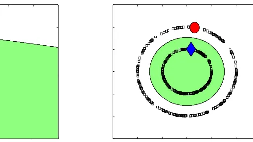
Figure 1: Unlabeled data and prior beliefs

examples may force us to restructure our hypotheses during learning. Imagine a situation where one is given two labeled examples—one positive and one negative—as shown in the left panel. If one is to induce a classifier on the basis of this, a natural choice would seem to be the linear separator as shown. Indeed, a variety of theoretical formalisms (Bayesian paradigms, regularization, minimum description length or structural risk minimization principles, and the like) have been constructed to rationalize such a choice. In most of these formalisms, one structures the set of one’s hypothesis functions by a prior notion of simplicity and one may then justify why the linear separator is the simplest structure consistent with the data.

Now consider the situation where one is given additional unlabeled examples as shown in the right panel. We argue that it is self-evident that in the light of this new unlabeled set, one must re-evaluate one’s prior notion of simplicity. The particular geometric structure of the marginal distribution suggests that the most natural classifier is now the circular one indicated in the right panel. Thus the geometry of the marginal distribution must be incorporated in our regularization principle to impose structure on the space of functions in nonparametric classification or regression. This is the intuition we formalize in the rest of the paper. The success of our approach depends on whether we can extract structure from the marginal distribution, and on the extent to which such structure may reveal the underlying truth.

1.2 Outline of the Paper

we consider the cases of fully supervised and unsupervised learning. In Section 7 we conclude this paper.

2. The Semi-Supervised Learning Framework

Recall the standard framework of learning from examples. There is a probability distribution P on X_×Raccording to which examples are generated for function learning. Labeled examples are (x,y)pairs generated according to P. Unlabeled examples are simply x_∈X drawn according to the

marginal distribution

P

X of P.

One might hope that knowledge of the marginal

P

Xcan be exploited for better function learning (e.g., in classification or regression tasks). Of course, if there is no identifiable relation between

P

X and the conditional

P

(y_|x), the knowledge of

P

X is unlikely to be of much use.

Therefore, we will make a specific assumption about the connection between the marginal and the conditional distributions. We will assume that if two points x1,x2∈X are close in the intrinsic

geometry of

P

X, then the conditional distributions

P

(y|x1)and

P

(y|x2)are similar. In other words,

the conditional probability distribution

P

(y_|x)varies smoothly along the geodesics in the intrinsic geometry of

P

X.

We use these geometric intuitions to extend an established framework for function learning. A number of popular algorithms such as SVM, Ridge regression, splines, Radial Basis Functions may be broadly interpreted as regularization algorithms with different empirical cost functions and complexity measures in an appropriately chosen Reproducing Kernel Hilbert Space (RKHS).

For a Mercer kernel K : X_×X_→R, there is an associated RKHS

H

K of functions X→Rwith the corresponding norm _{k k}K. Given a set of labeled examples (xi,yi), i=1, . . . ,l the standard framework estimates an unknown function by minimizing

f∗=argmin

f_∈HK

1

l l

∑

i=1

V(xi,yi,f) +γkfk2K, (1)

where V is some loss function, such as squared loss(yi−f(xi))2 for RLS or the hinge loss func-tion max[0,1−yif(xi)]for SVM. Penalizing the RKHS norm imposes smoothness conditions on possible solutions. The classical Representer Theorem states that the solution to this minimization problem exists in

H

K and can be written as

f∗(x) = l

∑

i=1

αiK(xi,x).

Therefore, the problem is reduced to optimizing over the finite dimensional space of coefficients αi, which is the algorithmic basis for SVM, regularized least squares and other regression and classification schemes.

We first consider the case when the marginal distribution is already known.

2.1 Marginal

P

X is Known

regularizer:

f∗=argmin

f∈HK

1

l l

∑

i=1

V(xi,yi,f) +γAkfk2K+γIkfk2I, (2) where_kf_k2_I is an appropriate penalty term that should reflect the intrinsic structure of

P

X. Intuitively,

kf_k2_I is a smoothness penalty corresponding to the probability distribution. For example, if the probability distribution is supported on a low-dimensional manifold, _kf_k2_I may penalize f along that manifold. γA controls the complexity of the function in the ambient space while γI controls the complexity of the function in the intrinsic geometry of

P

X. It turns out that one can derive an explicit functional form for the solution f∗as shown in the following theorem.

Theorem 1 Assume that the penalty term_kf_kIis sufficiently smooth with respect to the RKHS norm

kfkK(see Section 3.2 for the exact statement). Then the solution f∗to the optimization problem in Equation 2 above exists and admits the following representation

f∗(x) = l

∑

i=1

αiK(xi,x) +

Z

M α(z)K(x,z)d

P

X(z) (3)

where

M

=supp_{

P

X}is the support of the marginal

P

X.

We postpone the proof and the formulation of smoothness conditions on the norm_{k k}Iuntil the next section.

The Representer Theorem above allows us to express the solution f∗ directly in terms of the labeled data, the (ambient) kernel K, and the marginal

P

X. If

P

Xis unknown, we see that the solution may be expressed in terms of an empirical estimate of

P

X. Depending on the nature of this estimate, different approximations to the solution may be developed. In the next section, we consider a particular approximation scheme that leads to a simple algorithmic framework for learning from labeled and unlabeled data.

2.2 Marginal

P

X Unknown

In most applications the marginal

P

X is not known. Therefore we must attempt to get empirical estimates of

P

X andk kI. Note that in order to get such empirical estimates it is sufficient to have unlabeled examples.

A case of particular recent interest (for example, see Roweis and Saul, 2000; Tenenbaum et al., 2000; Belkin and Niyogi, 2003a; Donoho and Grimes, 2003; Coifman et al., 2005, for a discussion on dimensionality reduction) is when the support of

P

X is a compact submanifold

M

⊂Rn. In that case, one natural choice for_kf_kI is

R

x∈Mk∇M fk2d

P

X(x), where∇M is the gradient (see, for example Do Carmo, 1992, for an introduction to differential geometry) of f along the manifold

M

and the integral is taken over the marginal distribution.

The optimization problem becomes

f∗=argmin

f∈HK

1

l l

∑

i=1

V(xi,yi,f) +γAkfk2K+γI

Z

x∈Mk∇M fk

2_d

_P

X(x).

The termR

beyond the scope of this paper, it can be shown that under certain conditions choosing exponential weights for the adjacency graph leads to convergence of the graph Laplacian to the Laplace-Beltrami operator∆_M (or its weighted version) on the manifold. See the Remarks below and Belkin (2003); Lafon (2004); Belkin and Niyogi (2005); Coifman et al. (2005); Hein et al. (2005) for details.

Thus, given a set of l labeled examples_{(xi,yi)}l_i=1and a set of u unlabeled examples{xj}j_j=₌l_l+₊u₁, we consider the following optimization problem:

f∗=argmin

f∈HK

1

l l

∑

i=1

V(xi,yi,f) +γAkfk2K+ γI (u+l)2

l+u

∑

i,j=1

(f(xi)−f(xj))2Wi j,

=argmin

f∈HK

1

l l

∑

i=1

V(xi,yi,f) +γAkfk2K+ γI (u+l)2f

T_{Lf. (4)}

where Wi j are edge weights in the data adjacency graph, f= [f(x1), . . . ,f(xl+u)]T, and L is the graph Laplacian given by L=D₋W . Here, the diagonal matrix D is given by Dii=∑lj+=u1Wi j. The normalizing coefficient _(u+1_l)2 is the natural scale factor for the empirical estimate of the Laplace operator. We note than on a sparse adjacency graph it may be replaced by∑l_i,+_j=u₁Wi j.

The following version of the Representer Theorem shows that the minimizer has an expansion in terms of both labeled and unlabeled examples and is a key to our algorithms.

Theorem 2 The minimizer of optimization problem 4 admits an expansion

f∗(x) =

l+u

∑

i=1

αiK(xi,x) (5)

in terms of the labeled and unlabeled examples.

The proof is a variation of the standard orthogonality argument and is presented in Section 3.4.

Remark 1: Several natural choices of_{k k}I exist. Some examples are:

1. Iterated Laplacians(∆_M)k_{. Differential operators(}∆

M)k and their linear combinations pro-vide a natural family of smoothness penalties.

Recall that the Laplace-Beltrami operator∆_M can be defined as the divergence of the gradient vector field∆_M f=div(∇_M f)and is characterized by the equality

Z

x∈M f(x)∆Mf(x)dµ=

Z

x∈M k∇M f(x)k

2_dµ.

where µ is the standard measure (uniform distribution) on the Riemannian manifold. If µ is taken to be non-uniform, then the corresponding notion is the weighted Laplace-Beltrami operator (e.g., Grigor’yan, 2006).

2. Heat semigroup e−t∆M _{is a family of smoothing operators corresponding to the process of}

diffusion (Brownian motion) on the manifold. One can take_kf_k2_I =R

3. Squared norm of the Hessian (cf. Donoho and Grimes, 2003). While the Hessian H(f)(the matrix of second derivatives of f ) generally depends on the coordinate system, it can be shown that the Frobenius norm (the sum of squared eigenvalues) of H is the same in any geodesic coordinate system and hence is invariantly defined for a Riemannian manifold

M

. Using the Frobenius norm of H as a regularizer presents an intriguing generalization of thin-plate splines. We also note that∆_M(f) =tr(H(f)).

Remark 2: Why not just use the intrinsic regularizer? Using ambient and intrinsic regularizers

jointly is important for the following reasons:

1. We do not usually have access to

M

or the true underlying marginal distribution, just to data points sampled from it. Therefore regularization with respect only to the sampled manifold is ill-posed. By including an ambient term, the problem becomes well-posed.

2. There may be situations when regularization with respect to the ambient space yields a better solution, for example, when the manifold assumption does not hold (or holds to a lesser degree). Being able to trade off these two regularizers may be important in practice.

Remark 3: While we use the graph Laplacian for simplicity, the normalized Laplacian

˜L=D−1/2LD−1/2

can be used interchangeably in all our formulas. Using ˜L instead of L provides certain theoretical guarantees (see von Luxburg et al., 2004) and seems to perform as well or better in many practical tasks. In fact, we use ˜L in all our empirical studies in Section 5. The relation of ˜L to the weighted Laplace-Beltrami operator was discussed in Lafon (2004).

Remark 4: Note that a global kernel K restricted to

M

(denoted by K_M) is also a kernel defined on

M

with an associated RKHS

H

_M of functions

M

_→R. While this might suggest

kf_kI=kf_MkK_M

( f_M is f restricted to

M

) as a reasonable choice for_kf_kI, it turns out, that for the minimizer f∗of the corresponding optimization problem we get_kf∗_kI=kf∗kK, yielding the same solution as standard regularization, although with a different parameterγ. This observation follows from the restriction properties of RKHS discussed in the next section and is formally stated as Proposition 6. Therefore it is impossible to have an out-of-sample extension without two different measures of smoothness. On the other hand, a different ambient kernel restricted to

M

can potentially serve as the intrinsic regularization term. For example, a sharp Gaussian kernel can be used as an approximation to the heat kernel on

M

. Thus one (sharper) kernel may be used in conjunction with unlabeled data to estimate the heat kernel on

M

and a wider kernel for inference.

3. Theoretical Underpinnings and Results

3.1 General Theory of RKHS

We start by recalling some basic properties of reproducing kernel Hilbert spaces (see the original work of Aronszajn, 1950; Cucker and Smale, 2002, for a nice discussion in the context of learning theory) and their connections to integral operators. We say that a Hilbert space

H

of functions

X _→Rhas the reproducing property, if_∀x_∈X the evaluation functional f _→ f(x) is continuous. For the purposes of this discussion we will assume that X is compact. By the Riesz representation theorem it follows that for a given x_∈X , there is a function hx∈

H

, s.t.

∀f _∈

H

_hhx,fi_H = f(x).

We can therefore define the corresponding kernel function

K(x,y) =_hhx,hyi_H.

It follows that hx(y) =_hhx,hyi_H =K(x,y)and thushK(x,·),fi= f(x). It is clear that K(x,·)∈

H

. It is easy to see that K(x,y)is a positive semi-definite kernel as defined below:

Definition: We say that K(x,y), satisfying K(x,y) =K(y,x), is a positive semi-definite kernel if given an arbitrary finite set of points x1, . . . ,xn, the corresponding n×n matrix K with Ki j=K(xi,xj) is positive semi-definite.

Importantly, the converse is also true. Any positive semi-definite kernel K(x,y) gives rise to an RKHS

H

K, which can be constructed by considering the space of finite linear combina-tions of kernels ∑αiK(xi,·) and taking completion with respect to the inner product given by

hK(x,_·),K(y,_·)_iH

K=K(x,y). See Aronszajn (1950) for details.

We therefore see that reproducing kernel Hilbert spaces of functions on a space X are in

one-to-one correspondence with positive semidefinite kernels on X .

It can be shown that if the space

H

K is sufficiently rich, that is if for any distinct point x1, . . . ,xn there is a function f , s.t. f(x1) =1,f(xi) =0,i>1, then the corresponding matrix Ki j =K(xi,xj) is strictly positive definite. For simplicity we will sometimes assume that our RKHS are rich (the corresponding kernels are sometimes called universal).

Notation: In what follows, we will use kernel K to denote inner products and norms in the

cor-responding Hilbert space

H

K, that is, we will writeh , iK,k kK, instead of the more cumbersome

h , _iH

K,k kHK.

We proceed to endow X with a measure µ (supported on all of X ). The corresponding

L

_µ2Hilbert space inner product is given by

hf,g_iµ=

Z

X

f(x)g(x)dµ.

We can now consider the integral operator LKcorresponding to the kernel K:

(LKf)(x) =

Z

X

f(y)K(x,y)dµ.

It is well-known that if X is a compact space, LK is a compact operator and is self-adjoint with respect to

L

_µ2. By the spectral theorem, its eigenfunctions e1(x),e2(x), . . ., (scaled to norm 1) form an

orthonormal basis of

L

_µ2. The spectrum of the operator is discrete and the corresponding eigenvalues λ1,λ2, . . .are of finite multiplicity, limi→∞λi=0.

We see that

and therefore K(x,y) =∑_iλiei(x)ei(y). Writing a function f in that basis, we have f=∑aiei(x)and

hK(x,_·),f(_·)_iµ=∑iλiaiei(x).

It is not hard to show that the eigenfunctions eiare in

H

K (e.g., see the argument below). Thus we see that

ej(x) =_hK(x,_·),ej(_·)_iK=

∑

i

λiei(x)hei,eji_K.

Therefore _hei,ejiK=0, if i6= j, and hei,eiiK= λ1i. On the other hand hei,ejiµ=0, if i6= j, and

hei,eiiµ=1.

This observation establishes a simple relationship between the Hilbert norms in

H

Kand

L

µ2. We also see that f =∑aiei(x)∈

H

K if and only if∑a

2

i

λi <∞.

Consider now the operator L1_K/2. It can be defined as the only positive definite self-adjoint operator, s.t. LK=L1K/2◦L

1/2

K . Assuming that the series ˜K(x,y) =∑i

√_λ

iei(x)ei(y) converges, we can write

(L1_K/2f)(x) =

Z

X

f(y)_K˜_(x,y)dµ.

It is easy to check that L1_K/2is an isomorphism between

H

and

L

_µ2, that is ∀f,g_∈

H

K hf,gi_µ=hL1_K/2f,L1_K/2gi_K. Therefore

H

K is the image of L1K/2acting on

L

µ2.

Lemma 3 A function f(x) =∑_iaiei(x)can be represented as f=LKg for some g if and only if

∞

∑

i=1

a2_i

λ2

i

<∞. (6)

Proof Suppose f =LKg. Write g(x) =∑ibiei(x). We know that g∈L2µ if and only if ∑ib2i <∞. Since LK(∑ibiei) =∑ibiλiei=∑iaiei, we obtain ai=biλi. Therefore∑∞i=1

a2

i

λ2

i <∞.

Conversely, if the condition in the inequality 6 is satisfied, f =Lkg, where g=∑_λai_iei.

3.2 Proof of Theorems

Now let us recall the Equation 2:

f∗=argmin

f∈HK

1

l l

∑

i=1

V(xi,yi,f) +γAkfk2K+γIkfk2I.

We have an RKHS

H

K and the probability distribution µ which is supported on

M

⊂X . We denote by

S

the linear space, which is the closure with respect to the RKHS norm of

H

K, of the linear span of kernels centered at points of

M

:

Notation. By the subscript

M

we will denote the restriction to

M

. For example, by

S

_M we denote functions in

S

restricted to the manifold

M

. It can be shown (Aronszajn, 1950, p. 350) that the space(

H

K)M of functions from

H

Krestricted to

M

is an RKHS with the kernel KM, in other words (

H

K)M =

H

K_M.

Lemma 4 The following properties of

S

hold:

1.

S

with the inner product induced by

H

K is a Hilbert space.

2.

S

_M = (

H

K)M.

3. The orthogonal complement

S

⊥to

S

in

H

K consists of all functions vanishing on

M

.

Proof

1. From the definition of

S

it is clear by that

S

is a complete subspace of

H

K.

2. We give a convergence argument similar to the one found in Aronszajn (1950). Since (

H

K)M =

H

K_M any function fM in it can be written as fM = limn→∞fM,n, where

f_M,n=∑iαinK_M(xin,·)is a sum of kernel functions.

Consider the corresponding sum fn=∑iαinK(xin,·). From the definition of the norm we see that_kfn−fkkK =kfM,n−fM,kkK_M and therefore fn is a Cauchy sequence. Thus f =limn→∞fn exists and its restriction to

M

must equal f_M. This shows that(

H

K)_M ⊂

S

_M. The other direction follows by a similar argument.

3. Let g_∈

S

⊥. By the reproducing property for any x_∈

M

, g(x) =_hK(x,_·),g(_·)_iK=0 and there-fore any function in

S

⊥ vanishes on

M

. On the other hand, if g vanishes on

M

it is perpendicular to each K(x,_·),x_∈

M

and is therefore perpendicular to the closure of their span

S

.

Lemma 5 Assume that the intrinsic norm is such that for any f,g_∈

H

K,(f−g)|M ≡0 implies that

kf_kI=kgkI. Then assuming that the solution f∗of the optimization problem in Equation 2 exists, f∗_∈

S

.

Proof Any f _∈

H

Kcan be written as f = fS+f_S⊥, where fS is the projection of f to

S

and f_S⊥is its orthogonal complement.

For any x_∈M we have K(x,_·)_∈

S

. By the previous Lemma f_S⊥ vanishes on

M

. We have

f(xi) = fS(xi) _∀i and by assumptionkfSkI=kfkI.

On the other hand, _kf_k2_K=_kf_Sk2_K+_kf_S⊥_k2_K and therefore_kf_kK ≥ kfSkK. It follows that the minimizer f∗is in

S

.

As a direct corollary of these consideration, we obtain the following

Proposition 6 If_kf_kI=kfkK_M then the minimizer of Equation 2 is identical to that of the usual regularization problem (Equation 1) although with a different regularization parameter (λA+λI).

We can now restrict our attention to the study of

S

. While it is clear that the right-hand side of Equation 3 lies in

S

, not every element in

S

can be written in that form. For example, K(x,_·), where

x is not one of the data points xicannot generally be written as

l

∑

i=1

αiK(xi,x) +

Z

We will now assume that for f ∈

S

kf_k2_I =_hf,D f_iL2

µ.

We usually assume that D is an appropriate smoothness penalty, such as an inverse integral operator or a differential operator, for example, D f =∆_M f . The Representer theorem, however, holds under

quite mild conditions on D:

Theorem 7 Let_kf_k2

I =hf,D fiL2

µ where D is a bounded operator D :

S

→

L

2

PX. Then the solution

f∗of the optimization problem in Equation 2 exists and can be written as

f∗(x) = l

∑

i=1

αiK(xi,x) +

Z

Mα(y)K(x,y)d

P

X(y). (7)

Proof

For simplicity we will assume that the loss function V is differentiable. This condition can ultimately be eliminated by approximating a non-differentiable function appropriately and passing to the limit.

Put

H(f) =1 l

l

∑

i=1

V(xi,yi,f(xi)) +γAkfk2K+γIkfk2I.

We first show that the solution to Equation 2, f∗, exists and by Lemma 5 belongs to

S

. It follows easily from Cor. 10 and standard results about compact embeddings of Sobolev spaces (e.g., Adams, 1975) that a ball

B

r⊂

H

K,

B

r={f ∈

S

,s.t.kfkK ≤r}is compact in

L

X∞. Therefore for any such ball the minimizer in that ball f_r∗must exist and belong to

B

r. On the other hand, by substituting the zero function

H(f_r∗)_≤H(0) = 1 l

l

∑

i=1

V(xi,yi,0).

If the loss is actually zero, then zero function is a solution, otherwise

γAkfr∗k2K< l

∑

i=1

V(xi,yi,0),

and hence f_r∗_∈

B

r, where

r= s

∑l

i=1V(xi,yi,0)

γA

.

Therefore we cannot decrease H(f∗) by increasing r beyond a certain point, which shows that

f∗= f_r∗with r as above, which completes the proof of existence. If V is convex, such solution will also be unique.

We proceed to derive the Equation 7. As before, let e1,e2, . . . be the basis associated to the

integral operator(LKf)(x) =R_M f(y)K(x,y)d

P

X(y). Write f∗=∑iaiei(x). By substituting f∗into H(f)we obtain:

H(f∗) =1 l

l

∑

j=1

V(xj,yj,

∑

i

Assume that V is differentiable with respect to each ak. We havek∑iaiei(x)k2K=∑i

a2

i

λi.

Differenti-ating with respect to the coefficients aiyields the following set of equations:

0=∂H(f∗) ∂ak

=1 l

l

∑

j=1

ek(xj)∂3V(xj,yj,

∑

i

aiei) +2γA ak λk

+γIhD f,eki+γIhf,Deki,

where∂3V denotes the derivative with respect to the third argument of V .

hD f,eki+hf,Deki=h(D+D∗)f,ekiand hence

ak=− λk 2γAl

l

∑

j=1

ek(xj)∂3V(xj,yj,f∗)− γI 2γA

λkhD f∗+D∗f∗,eki.

Since f∗(x) =∑_kakek(x)and recalling that K(x,y) =∑iλiei(x)ei(y)

f∗(x) =₋ 1 2γAl

∑

_k

l

∑

j=1

λkek(x)ek(xj)∂3V(xj,yj,f∗)− γI 2γA

∑

_k

λkhD f∗+D∗f∗,ekiek,

=₋ 1

2γAl l

∑

j=1

K(x,xj)∂3V(xj,yj,f∗)− γI 2γA

∑

_k

λkhD f∗+D∗f∗,ekiek.

We see that the first summand is a sum of the kernel functions centered at data points. It re-mains to show that the second summand has an integral representation, that is, can be written as

R

Mα(y)K(x,y)d

P

X(y), which is equivalent to being in the image of LK. To verify this we apply Lemma 3. We need that

∑

k

λ2

khD f∗+D∗f∗,eki

2

λ2

k

=

∑

k

hD f∗+D∗f∗,eki2<∞.

Since D, its adjoint operator D∗ and hence their sum are bounded the inequality above is satisfied for any function in

S

.

3.3 Manifold Setting2

We now show that for the case when

M

is a manifold and D is a differential operator, such as the Laplace-Beltrami operator∆_M, the boundedness condition of Theorem 7 is satisfied. While we consider the case when the manifold has no boundary, the same argument goes through for manifold with boundary, with, for example, Dirichlet’s boundary conditions (vanishing at the boundary). Thus the setting of Theorem 7 is very general, applying, among other things, to arbitrary differential operators on compact domains in Euclidean space.

Let

M

be a

C

∞manifold without boundary with an infinitely differentiable embedding in some ambient space X , D a differential operator with

C

∞ coefficients and let µ, be the measure corre-sponding to some

C

∞nowhere vanishing volume form on

M

. We assume that the kernel K(x,y)is also infinitely differentiable.3 As before for an operator A, A∗denotes the adjoint operator.

2. We thank Peter Constantin and Todd Dupont for help with this section.

3. While we have assumed that all objects are infinitely differentiable, it is not hard to specify the precise differentiability conditions. Roughly speaking, a degree k differential operator D is bounded as an operatorHK→L2µ, if the kernel

Theorem 8 Under the conditions above D is a bounded operator

S

→

L

2

µ.

Proof First note that it is enough to show that D is bounded on

H

K_M, since D only depends on the restriction f_M. As before, let LK_M(f)(x) =R_M f(y)K_M(x,y)dµ is the integral operator associated to KM. Note that D∗is also a differential operator of the same degree as D. The integral operator LK_M is bounded (compact) from L2µto any Sobolev space Hsob. Therefore the operator LK_MD is also bounded. We therefore see that DLK_MD∗is bounded L2µ→L2µ. Therefore there is a constant C, s.t.

hDLK_MD∗f,fiL2

µ ≤CkfkL2µ.

The square root T =L_K1/2

M of the self-adjoint positive definite operator LKM is a self-adjoint

positive definite operator as well. Thus(DT)∗_{=T D}∗_{. By definition of the operator norm, for any}

ε>0 there exists f _∈L2_µ,_kf_kL2

µ≤1+ε, such that

kDT_k2_L2

µ=kT D ∗_k2

L2

µ ≤ hT D

∗_{f,T D}∗_fi

L2

µ =

=_hDLD∗f,f_iL2

µ ≤ kDLD ∗_k

L2

µkfk 2

L2

µ ≤C(1+ε) 2_.

Therefore the operator DT : L2_µ→L2_µis bounded (and also_kDT_kL2

µ ≤C, sinceεis arbitrary).

Now recall that T provides an isometry between L2_µand

H

K_M. That means that for any g∈

H

K_M there is f _∈L2_µ, such that T f =g and_kf_kL2

µ=kgkKM. ThuskDgkLµ2=kDT fkLµ2≤CkgkKM, which

shows that T :

H

K_M →L2µis bounded and concludes the proof.

Since

S

is a subspace of

H

Kthe main result follows immediately:

Corollary 9 D is a bounded operator

S

_→L2_µand the conditions of Theorem 7 hold.

Before finishing the theoretical discussion we obtain a useful

Corollary 10 The operator T=L1_K/2on L2

µis a bounded (and in fact compact) operator L2µ→Hsob, where Hsobis an arbitrary Sobolev space.

Proof Follows from the fact that DT is bounded operator L2_µ→L2_µfor an arbitrary differential op-erator D and standard results on compact embeddings of Sobolev spaces (see, for example, Adams, 1975).

3.4 The Representer Theorem for the Empirical Case

Proof (Theorem 2) Any function f ∈

H

Kcan be uniquely decomposed into a component f_||in the linear subspace spanned by the kernel functions_{K(xi,·)}li=+1u, and a component f⊥orthogonal to it.

Thus,

f = f_||+f_⊥=

l+u

∑

i=1

αiK(xi,·) +f⊥.

By the reproducing property, as the following arguments show, the evaluation of f on any data point xj, 1≤ j≤l+u is independent of the orthogonal component f⊥:

f(xj) =hf,K(xj,·)i=h

l+u

∑

i=1

αiK(xi,·),K(xj,·)i+hf⊥,K(xj,·)i.

Since the second term vanishes, and _hK(xi,·),K(xj,·)i = K(xi,xj), it follows that f(xj) =∑li=+1uαiK(xi,xj). Thus, the empirical terms involving the loss function and the intrinsic norm in the optimization problem in Equation 4 depend only on the value of the coefficients_{αi}l_i=+u₁ and the gram matrix of the kernel function.

Indeed, since the orthogonal component only increases the norm of f in

H

K:

kfk2

K=k

l+u

∑

i=1

αiK(xi,·)k2K+kf⊥k2K≥ k

l+u

∑

i=1

αiK(xi,·)k2K.

It follows that the minimizer of problem 4 must have f_⊥=0, and therefore admits a representation

f∗(_·) =∑l_i=+₁uαiK(xi,·).

The simple form of the minimizer, given by this theorem, allows us to translate our extrinsic and intrinsic regularization framework into optimization problems over the finite dimensional space of coefficients_{αi}l_i+₌₁u, and invoke the machinery of kernel based algorithms. In the next section, we derive these algorithms, and explore their connections to other related work.

4. Algorithms

We now discuss standard regularization algorithms (RLS and SVM) and present their extensions (LapRLS and LapSVM respectively). These are obtained by solving the optimization problems posed in Equation 4) for different choices of cost function V and regularization parametersγA,γI. To fix notation, we assume we have l labeled examples _{(xi,yi)}l_i=1 and u unlabeled examples

{xj}j_j=₌l_l+₊u₁. We use K interchangeably to denote the kernel function or the Gram matrix.

4.1 Regularized Least Squares

The regularized least squares algorithm is a fully supervised method where we solve:

min

f∈HK

1

l l

∑

i=1

(yi−f(xi))2+γkfk2K.

The classical Representer Theorem can be used to show that the solution is of the following form:

f?(x) = l

∑

i=1

α?

Substituting this form in the problem above, we arrive at following convex differentiable objec-tive function of the l-dimensional variableα= [α1. . .αl]T:

α∗_=argmin1

l(Y−Kα)

T_(Y

−Kα) +γαTKα,

where K is the l_×l gram matrix Ki j=K(xi,xj)and Y is the label vector Y = [y1. . .yl]T. The derivative of the objective function vanishes at the minimizer:

1

l(Y−Kα

∗₎T₍

−K) +γKα∗=0,

which leads to the following solution:

α∗_{= (K+γlI)}−1_Y.

4.2 Laplacian Regularized Least Squares (LapRLS)

The Laplacian regularized least squares algorithm solves the optimization problem in Equation 4) with the squared loss function:

min

f∈HK

1

l l

∑

i=1

(yi−f(xi))2+γAkfk2K+ γI (u+l)2f

T_Lf.

As before, the Representer Theorem can be used to show that the solution is an expansion of kernel functions over both the labeled and the unlabeled data:

f?(x) =

l+u

∑

i=1

α?

iK(x,xi).

Substituting this form in the equation above, as before, we arrive at a convex differentiable objective function of the l+u-dimensional variableα= [α1. . .αl+u]T:

α∗_=argmin

α∈Rl+u

1

l(Y−JKα)

T_(Y

−JKα) +γAαTKα+ γI (u+l)2α

T_KLKα,

where K is the (l+u)_×(l+u) Gram matrix over labeled and unlabeled points; Y is an (l+u) dimensional label vector given by: Y = [y1, . . . ,yl,0, . . . ,0]and J is an(l+u)×(l+u) diagonal matrix given by J=diag(1, . . . ,1,0, . . . ,0)with the first l diagonal entries as 1 and the rest 0.

The derivative of the objective function vanishes at the minimizer:

1

l(Y−JKα)

T₍

−JK) + (γAK+ γIl

(u+l)2KLK)α=0,

which leads to the following solution:

α∗_{= (JK+γ}

AlI+

γIl

(u+l)2LK)−

1_{Y. (8)}

4.3 Support Vector Machine Classification

Here we outline the SVM approach to binary classification problems. For SVMs, the following problem is solved:

min

f_∈HK

1

l l

∑

i=1

(1₋yif(xi))++γkfk2K,

where the hinge loss is defined as:(1₋y f(x))+=max(0,1−y f(x))and the labels yi∈ {−1,+1}. Again, the solution is given by:

f?(x) = l

∑

i=1

α?

iK(x,xi). (9)

Following SVM expositions, the above problem can be equivalently written as:

min

f∈HK,ξi∈R

1

l l

∑

i=1

ξi+γkfk2K subject to: yif(xi)≥1−ξi i=1, . . . ,l ξi≥0 i=1, . . . ,l.

Using the Lagrange multipliers technique, and benefiting from strong duality, the above problem has a simpler quadratic dual program in the Lagrange multipliersβ= [β1, . . . ,βl]T ∈Rl:

β? _{= max}

β∈Rl

l

∑

i=1

βi− 1 2β

T_Qβ

subject to:

l

∑

i=1

yiβi=0

0≤βi≤ 1

l i=1, . . . ,l.

where the equality constraint arises due to an unregularized bias term that is often added to the sum in Equation 9, and the following notation is used:

Y = diag(y1,y2, ...,yl),

Q = Y

K

2γ

Y,

α? ₌ Yβ?

2γ .

4.4 Laplacian Support Vector Machines

By including the intrinsic smoothness penalty term, we can extend SVMs by solving the following problem:

min

f_∈HK

1

l l

∑

i=1

(1₋yif(xi))++γAkfk2K+ γI (u+l)2f

T_Lf.

By the representer theorem,as before, the solution to the problem above is given by:

f?(x) =

l+u

∑

i=1

α?

iK(x,xi).

Often in SVM formulations, an unregularized bias term b is added to the above form. Again, the primal problem can be easily seen to be the following:

min α∈Rl+u_,ξ_∈Rl

1

l l

∑

i=1

ξi+γAαTKα+ γI (u+l)2α

T_KLKα

subject to: yi(

l+u

∑

j=1

αjK(xi,xj) +b)≥1−ξi, i=1, . . . ,l

ξi≥0 i=1, . . . ,l.

Introducing the Lagrangian, withβi,ζias Lagrange multipliers:

L(α,ξ,b,β,ζ) = 1 l

l

∑

i=1

ξi+ 1 2α

T_(2γ

AK+2

γA

(l+u)2KLK)α

−

l

∑

i=1

βi(yi(

l+u

∑

j=1

αjK(xi,xj) +b)−1+ξi)− l

∑

i=1

ζiξi.

Passing to the dual requires the following steps:

∂L

∂b =0 =⇒ l

∑

i=1

βiyi=0,

∂L

∂ξi

=0 =_⇒ 1

l −βi−ζi=0,

=_⇒ 0≤βi≤ 1

l (ξi,ζiare non-negative).

Using above identities, we formulate a reduced Lagrangian:

LR(α,β) = 1 2α

T_(2γ

AK+2

γI

(u+l)2KLK)α−

l

∑

i=1

βi(yi

l+u

∑

j=1

αjK(xi,xj)−1),

= 1

2α

T_(2γ

AK+2

γI

(u+l)2KLK)α−α

T_KJT_Yβ+

∑

l

i=1

where J= [I 0]is an l×(l+u)matrix with I as the l×l identity matrix (assuming the first l points

are labeled) and Y=diag(y1,y2, ...,yl).

Taking derivative of the reduced Lagrangian with respect toα:

∂LR

∂α = (2γAK+2 γI

(u+l)2KLK)α−KJ

T_Yβ.

This implies:

α= (2γAI+2 γI

(u+l)2LK)−

1_JT_Yβ?_{. (10)}

Note that the relationship between α andβis no longer as simple as the SVM algorithm. In particular, the(l+u)expansion coefficients are obtained by solving a linear system involving the l dual variables that will appear in the SVM dual problem.

Substituting back in the reduced Lagrangian we get:

β∗ _{= max}

β∈Rl

l

∑

i=1

βi− 1 2β

T_{Qβ (11)}

subject to:

l

∑

i=1

βiyi=0

0_≤βi≤ 1

l i=1, . . . ,l (12)

where

Q=Y JK(2γAI+2 γI

(l+u)2LK)− 1_JT_Y.

Laplacian SVMs can be implemented by using a standard SVM solver with the quadratic form induced by the above matrix, and using the solution to obtain the expansion coefficients by solving the linear system in Equation 10.

Note that whenγI=0, the SVM QP and Equations 11 and 10, give zero expansion coefficients over the unlabeled data. The expansion coefficients over the labeled data and the Q matrix are as in standard SVM, in this case.

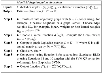
The manifold regularization algorithms are summarized in the Table 1.

Efficiency Issues: It is worth noting that our algorithms compute the inverse of a dense Gram matrix

which leads to O((l+u)3_{)complexity. This may be impractical for large data sets. In the case of}

linear kernels, instead of using Equation 5, we can directly write f?(x) =wTx and solve for the

Manifold Regularization algorithms

Input: l labeled examples{(xi,yi)}li=1, u unlabeled examples{xj}l_j+₌u_l+1

Output: Estimated function f :Rn→R

Step 1 Construct data adjacency graph with (l+u) nodes using, for

example, k nearest neighbors or a graph kernel. Choose edge weights Wi j, for example, binary weights or heat kernel weights Wi j=e−kxi−xjk

2_/4t

.

Step 2 _{Choose a kernel function K}(_x,_y)_{. Compute the Gram matrix}

Ki j=K(xi,xj).

Step 3 Compute graph Laplacian matrix: L=D−W where D is a

di-agonal matrix given by Dii=∑l_j+₌u₁Wi j.

Step 4 Chooseγ_Aandγ_I.

Step 5 _Computeα∗_{using Equation 8 for squared loss (Laplacian RLS)}

or using Equations 11 and 10 together with the SVM QP solver for soft margin loss (Laplacian SVM).

Step 6 Output function f∗(x) =∑l+u

i=1α∗iK(xi,x).

Table 1: A summary of the algorithms

scalability issues in semi-supervised learning, see, example, Tsang and Kwok. (2005); Bengio et al. (2004).

4.5 Related Work and Connections to Other Algorithms

In this section we survey various approaches to semi-supervised and transductive learning and high-light connections of manifold regularization to other algorithms.

Transductive SVM (TSVM) (Vapnik, 1998; Joachims, 1999): TSVMs are based on the

follow-ing optimization principle:

f∗= argmin

f∈HK

yl+1,...yl+u

C l

∑

i=1

(1−yif(xi))++C∗

l+u

∑

i=l+1

(1−yif(xi))++kfk2K,

which proposes a joint optimization of the SVM objective function over binary-valued labels on the unlabeled data and functions in the RKHS. Here, C,C∗are parameters that control the relative hinge-loss over labeled and unlabeled sets. The joint optimization is implemented in Joachims (1999) by first using an inductive SVM to label the unlabeled data and then iteratively solving SVM quadratic programs, at each step switching labels to improve the objective function. However this procedure is susceptible to local minima and requires an unknown, possibly large number of label switches before converging. Note that even though TSVM were inspired by transductive inference, they do provide an out-of-sample extension.

labels for each unlabeled example. This is formulated as a mixed-integer program for linear SVMs in Bennett and Demiriz (1999) and is found to be intractable for large amounts of unlabeled data. Fung and Mangasarian (2001) reformulate this approach as a concave minimization problem which is solved by a successive linear approximation algorithm. The presentation of these algorithms is restricted to the linear case.

Measure-Based Regularization (Bousquet et al., 2004): The conceptual framework of this

work is closest to our approach. The authors consider a gradient based regularizer that penalizes variations of the function more in high density regions and less in low density regions leading to the following optimization principle:

f∗=argmin

f∈F

l

∑

i=1

V(f(xi),yi) +γ

Z

Xh∇

f(x),∇f(x)_ip(x)dx,

where p is the density of the marginal distribution

P

X. The authors observe that it is not straightfor-ward to find a kernel for arbitrary densities p, whose associated RKHS norm is

Z

h∇f(x),∇f(x)_ip(x)dx.

Thus, in the absence of a representer theorem, the authors propose to perform minimization of the regularized loss on a fixed set of basis functions chosen apriori, that is,

F

=_{∑q_i=1αiφi}. For the hinge loss, this paper derives an SVM quadratic program in the coefficients_{αi}q_i=1whose Q matrix is calculated by computing q2integrals over gradients of the basis functions. However the algorithm does not demonstrate performance improvements in real world experiments. It is also worth noting that while Bousquet et al. (2004) use the gradient∇f(x)in the ambient space, we use the gradient over a submanifold∇_M f for penalizing the function. In a situation where the data truly lies on

or near a submanifold

M

, the difference between these two penalizers can be significant since smoothness in the normal direction to the data manifold is irrelevant to classification or regression.

Graph-Based Approaches See, for example, Blum and Chawla (2001); Chapelle et al. (2003);

Szummer and Jaakkola (2002); Zhou et al. (2004); Zhu et al. (2003, 2005); Kemp et al. (2004); Joachims (2003); Belkin and Niyogi (2003b): A variety of graph-based methods have been pro-posed for transductive inference. However, these methods do not provide an out-of-sample exten-sion. In Zhu et al. (2003), nearest neighbor labeling for test examples is proposed once unlabeled examples have been labeled by transductive learning. In Chapelle et al. (2003), test points are approximately represented as a linear combination of training and unlabeled points in the feature space induced by the kernel. For graph regularization and label propagation see (Smola and Kondor, 2003; Belkin et al., 2004; Zhu et al., 2003). Smola and Kondor (2003) discusses the construction of a canonical family of graph regularizers based on the graph Laplacian. Zhu et al. (2005) presents a non-parametric construction of graph regularizers.

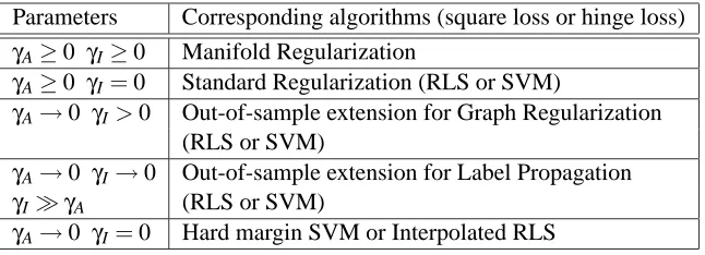
Manifold regularization provides natural out-of-sample extensions to several graph-based ap-proaches. These connections are summarized in Table 2.

We also note the recent work (Delalleau et al., 2005) on out-of-sample extensions for semi-supervised learning where an induction formula is derived by assuming that the addition of a test point to the graph does not change the transductive solution over the unlabeled data.

Cotraining (Blum and Mitchell, 1998): The cotraining algorithm was developed to integrate

subsets of unlabeled examples are used to mutually expand the training set. Note that this set-ting may not be applicable in several cases of practical interest where one does not have access to multiple information sources.

Bayesian Techniques See, for example, Nigam et al. (2000); Seeger (2001); Corduneanu and

Jaakkola (2003). An early application of semi-supervised learning to Text classification appeared in Nigam et al. (2000) where a combination of EM algorithm and Naive-Bayes classification is pro-posed to incorporate unlabeled data. Seeger (2001) provides a detailed overview of Bayesian frame-works for semi-supervised learning. The recent work in Corduneanu and Jaakkola (2003) formu-lates a new information-theoretic principle to develop a regularizer for conditional log-likelihood.

Parameters Corresponding algorithms (square loss or hinge loss) γA≥0 γI≥0 Manifold Regularization

γA≥0 γI=0 Standard Regularization (RLS or SVM)

γA→0 γI>0 Out-of-sample extension for Graph Regularization (RLS or SVM)

γA→0 γI→0 Out-of-sample extension for Label Propagation

γIγA (RLS or SVM)

γA→0 γI=0 Hard margin SVM or Interpolated RLS

Table 2: Connections of manifold regularization to other algorithms

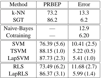
5. Experiments

We performed experiments on a synthetic data set and three real world classification problems aris-ing in visual and speech recognition, and text categorization. Comparisons are made with inductive methods (SVM, RLS). We also compare Laplacian SVM with transductive SVM. All software and data sets used for these experiments will be made available at:

http://www.cs.uchicago.edu/_∼vikass/manifoldregularization.html.

For further experimental benchmark studies and comparisons with numerous other methods, we refer the reader to Chapelle et al. (2006); Sindhwani et al. (2006, 2005).

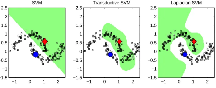
5.1 Synthetic Data: Two Moons Data Set

−1 0 1 2 −1

0 1 2

γ

A = 0.03125 γI = 0

SVM

−1 0 1 2

−1 0 1 2

Laplacian SVM

γ

A = 0.03125 γI = 0.01

−1 0 1 2

−1 0 1 2

Laplacian SVM

γ

A = 0.03125 γI = 1

Figure 2: Laplacian SVM with RBF kernels for various values ofγI. Labeled points are shown in color, other points are unlabeled.

−1 0 1 2

−1.5 −1 −0.5 0 0.5 1 1.5 2 2.5

SVM

−1 0 1 2

−1.5 −1 −0.5 0 0.5 1 1.5 2 2.5

Transductive SVM

−1 0 1 2

−1.5 −1 −0.5 0 0.5 1 1.5 2 2.5

Laplacian SVM

Figure 3: Two Moons data set: Best decision surfaces using RBF kernels for SVM, TSVM and Laplacian SVM. Labeled points are shown in color, other points are unlabeled.

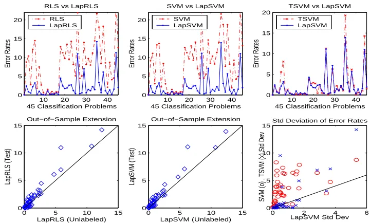
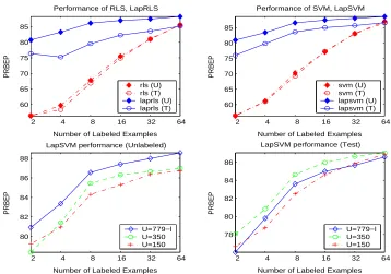
5.2 Handwritten Digit Recognition

In this set of experiments we applied Laplacian SVM and Laplacian RLS algorithms to 45 binary classification problems that arise in pairwise classification of handwritten digits. The first 400 im-ages for each digit in the USPS training set (preprocessed using PCA to 100 dimensions) were taken to form the training set. The remaining images formed the test set. 2 images for each class were randomly labeled (l=2) and the rest were left unlabeled (u=398). Following Scholkopf et al. (1995), we chose to train classifiers with polynomial kernels of degree 3, and set the weight on the regular-ization term for inductive methods asγl=0.05(C=10). For manifold regularization, we chose to split the same weight in the ratio 1 : 9 so thatγAl=0.005,_(u+γIl_l)2 =0.045. The observations reported in this section hold consistently across a wide choice of parameters.