Sanel Halilbegovic, Mia Vehabovic

(1)

Copyright © 2016 by Academic Publishing House Researcher

Published in the Russian Federation

European Journal of Economic Studies

Has been issued since 2012.

ISSN: 2304-9669 E-ISSN: 2305-6282

Vol. 17, Is. 3, pp. 393-404, 2016

DOI: 10.13187/es.2016.17.393

www.ejournal2.com

Articles and Statements

UDC 33

Backtesting Value at Risk Forecast: the Case of Kupiec Pof-Test

Sanel Halilbegovic a , *_{, Mia Vehabovic}a

a _{International Burch University, Sarajevo, Bosnia and Herzegovina}

Abstract

In recent years many concepts for managing and measuring risk have been developed. The main methodology for managing risk is a method of value at risk, which, in practice, is combined with other techniques for minimizing risks, in order to achieve optimal business results. Value at risk (VaR) is the biggest loss of the portfolio that can be expected in the reporting period, with a given level of confidence. This value is a simple, easily understandable number that presents the risk, which the institution is exposed to on financial market. The principle of calculating capital is based on the VaR methodology. However, back testing of calculated VaR amount is needed. Back testing is the process where the real gains and losses are compared to the forecasted VaR estimates. The most used back-testing test is known as Kupiec POF test. The POF's null hypothesis, that the observed failure rate is equal to the failure rate suggested by the confidence interval, is being tested using the secondary data (daily share prices from http://finance.yahoo.com). The results from the test show that, at 90 % and 99 % level of confidence, null hypothesis is rejected and the model is considered as inaccurate.

Keywords: value at risk, back testing, confidence interval, risk management, POF test.

1. Introduction

We are often in a position to make a decision without reviewing all the consequences and the uncertainties, which that decision can bring, and furthermore, in fact some of the consequences may be unfavourable. A precise definition of risk does not exist, but what is common to all definitions are uncertainty and loss. The risk means any uncertain situation in the business and the probability of loss (gain reduction) as a result of uncertain events in the business. The most famous type of risk that is related to the securities is market risk, which relates to the uncertainty regarding the change in the price of securities (Halilbegović, 2016).

(2)

institutions in their operations encounter. In their business, financial institutions nowadays face two major challenges: risk management and profit maximization. This represents a difficult task, since the risks are numerous and it is difficult to be identified and even more difficult to be controlled. Risk management has two main objectives:

1.) to improve the financial performance of the institution

2.) to ensure that the institution does not suffer unacceptable losses.

Financial institutions increase revenue by risk-taking and managing it. Therefore, for the profitability of the institution, the relationship between management of the risk and income is of crucial importance. Risk is defined as the general uncertainty of future outcomes, instability due to unexpected results. On the financial market there is a need to solve the problem of optimal investment in selected goods, under certain risk. Possible investments constitute portfolio, so the problem of optimizing the portfolio should be solved, which includes a measure of investment risk. The risk can be estimated using various measures of risk. The first ideas for assessing portfolio risk came from Markowitz, who measured the risk using mean variance behaviour. Two measures of risk later emerged: VaR (Value at Risk) and CVaR (Conditional Value at Risk). VaR has become the main measure of risk in banking regulations and in internal risk management of banks. VaR is much easier to calculate than most measures for risk and therefore takes an important position in practice. During 1996, 99 % VaR is accepted by the Basel Accord as the main measure of risk for determination of possible loss. It also became a central measure of the internal risk management of the banking system.

A significant role in the risk management of international banking and other financial sector has the Basel Committee on Banking Supervision. Basel became the generally accepted standard, significant for financial flows and investment policy. With this agreement, the term of the required minimum capital is introduced and defined, which must be met so that the bank protect itself against the risk (Jorion, 2001).

2. Literature review

Value at risk, VaR, is a measure of risk investment in the financial market. It is the greatest loss that can be expected in a given time interval, with a given level of confidence. It is important to note that the VaR is only an estimate of the possible loss. One of the advantages of VaR is that it is a simple, easily understandable number, which is a measure of risk to which the institution is exposed to in the financial market. The term VaR has never been recorded as a financial term until early 1990, but it actually originated many years ago. In fact, it could be said that the term derives from the need for safety of capital of US companies from the beginning of the twentieth century, starting with the implementation of the informal capital test. VaR has its roots in Markowitz's theory of portfolio. Specifically, the methodology underlying the VaR is a result of integrating modern portfolio theory and statistical analysis, which examines the risk factors. In 1998, banks began to use VaR as a measure of risk for calculating the necessary regulatory funds. VaR is introduced by Dennis Weatherstone, chairman of the US bank JP Morgan, with the aim to give him the opportunity to control the daily risk exposure of his company. He gave the task to his analysts to submit a report to him every day – which will be just a number, a number that indicates the potential loss of the day (Campbell, 2005). The participation of positions during the observed period in the portfolio is fixed, which means that VaR provides an opportunity to assess the potential loss (if the structure of the portfolio is not changed). Since it is a value that is calculated with a certain level of confidence, about the estimated loss is possible to speak only as of the

potential, and it cannot be said that this is a number that indicates the maximum extent of feasible and safe loss. Thus, VaR does not indicate potential losses in extreme market conditions. For example, if the level of confidence is 95 %, the calculated indicator says that it should not be lost more than the stated amount in 95 %; but does not tell what might happen in the remaining 5% of cases.

According to Jorion (2001) the formula for VaR is expressed as: VaR = a * * W (1) Variables in formula (1) are:

a – confidence interval

(3)

W – Initial portfolio value

VaR takes into consideration how changes in prices of financial instruments affect each other. Therefore, it can reduce the risk with the help of diversification. Although VaR is not an ideal solution in all situations, it certainly is an effective measure of market risk under normal market conditions. Thus, VaR is a measure of risk in the portfolio for the usual business, to a given level of confidence. Therefore, VaR is not efficient in terms of the extreme changes in the market and therefore it should be combined with stress tests, in order to obtain a wider framework for the observation of market risk. As emphasized in the paper What is the Best Risk Measure in Practice? A Comparison of Standard Measures (Emmer et al., 2015) the VaR is generally accepted, standard measure of market risk that regulatory institutions require banks to use in the calculation of the required of capital. There are three main methods for calculating VaR risk measures:

1) Parametric method (variance-covariance method)

In this method it is assumed that the market variables have a normal distribution and use its features to determine VaR. The main characteristic of the normal distribution is that its density function is symmetric and that is completely determined if two parameters are known: the mean and standard deviation. As Down, 1998 stated in his paper Retrospective Assessment of Value-at-Risk, one of the main problems of using the normal distribution to estimate VaR is its main advantage in the same time and it refers to the fact that the calculation requires only two parameters.

2)Method of historical simulation

The historical simulation belongs to the non-parametric method for calculating VaR. What is common to all the non-parametric approach is the usage of the empirical distribution, obtained from the observed data, as opposed to the parametric approach (where the assumptions about the theoretical distributions of return are used). The main characteristic of historical simulation is its implementation easiness (Wiener, 1999).

3) Monte-Carlo simulation method

Monte Carlo method is a method for generating random numbers. Using random numbers, various problems can be solved by simulation. The idea of Monte Carlo simulation is to simulate the appearance that is observed in order to obtain the realization of phenomena that cannot be obtained otherwise. The simulation is performed certain number times, and the collection of obtained realization presents statistical data set (Jorion, 2001).

(4)

Table 1. Backtesting types

For the purposes of backtesting process, the data representing the information about actual share prices of companies are available at http://finance.yahoo.com. Given that the data used for backtesting process is based on real information, therefore it is expected that the test results are realistic.

Hypothesis

The POF test (proportion of failure) examines whether the number of exceptions is in accordance with the level of confidence. The null hypothesis for the proportion of failure is expressed as:

H0: p = = (2) Variables in formula (2) are:

p - The proportion of failure - The observed failure rate X - Number of exceptions T - Number of observations

The null hypothesis states that the observed failure rate is equal to the failure rate, which is suggested by the confidence interval. Furthermore, the goal of accepting the null hypothesis is to prove that the model is accurate. In the case where the amount of likelihood ratio is greater than the critical value of the χ², the conclusion about rejecting the null hypothesis and model inaccuracy would be made.

3. Methodology

The main reason why this research has been written is that there are many discussions whether the VaR models are reliable or not. This study takes into consideration the basic test, the so-called POF Test, which stands for the proportion of failure, and measures whether the number of exceptions is in accordance with the level of confidence. The likelihood ratio test, „LR“ is expressed through the following formula:

LR POF= -2ln (3)

and according to Jorion, 2001 the exact definition of the likelihood ratio test is: “Likelihood-ratio test is a statistical test that calculates the ratio between the maximum probabilities of a result under two alternative hypotheses. The maximum probability of the observed result under null hypothesis is defined in the numerator and the maximum probability of the observed result under the alternative hypothesis is defined in the denominator. The decision is then based on the value of this ratio. The smaller the ratio is, the larger the LR-statistic will be. If the value becomes too

large compared to the critical value of χ² distribution, the null hypothesis is rejected. According to

statistical decision theory, likelihood-ratio test is the most powerful test in its class”. In the case where the amount of likelihood ratio is greater than the critical value of the χ², the conclusion about rejecting the null hypothesis and model inaccuracy would be made.

Backtesting Types

Unconditional Coverage Test Independence Test

(5)

Data used for those statistical calculations are from secondary source, more precisely, share prices for the period of 251 trading days are taken from http://finance.yahoo.com for five companies: Procter&Gamble, Mc Donalds, Microsoft, Caterpillar and Apple. First of all, daily returns are calculated for each company (without dividends), then daily return for portfolio is calculated in a way that daily returns from five companies are summed up.

The third step is the calculation of one day VaR for the porfolio at 90 %, 95 % and 99 % level of confidence by using the formula (1). Daily losses are then taken into consideration in order to compare these values with estimated VaR calculation. If the value of portfolio's loss is greater than the forecasted one day VaR value, the exception exists. This comparison is needed to see how many exceptions occur at 90 %, 95 % and 99 % level of confidence. Once the one day VaR and number of exceptions for each level of confidence are known; the likelihood ratio test is to be calculated by using formula (3). In the case that the calculated LR exceeds the critical value, the null hypothesis and model accuracy are to be rejected for certain level of confidence.

4. Data analysis and discussion

As already written in the methodology part, daily (close) prices for five companies are considered and presented in the Table 2 for the period of 251 working/trading days (05.08.2013. - 04.08.2014.):

Table 2. Daily prices

Date Procter&Gamble McD Microsoft Caterpillar Apple

4.8.2014 79.22 94.31 43.37 101.81 95.59

1.8.2014 79.65 94.30 42.86 100.52 96.13

31.7.2014 77.32 94.56 43.16 100.75 95.60

30.7.2014 78.16 95.95 43.58 103.38 98.15

29.7.2014 78.65 95.82 43.89 104.69 98.38

28.7.2014 79.26 95.78 43.97 104.15 99.02

25.7.2014 79.56 95.72 44.50 104.85 97.67

24.7.2014 80.26 95.35 44.40 105.04 97.03

23.7.2014 79.99 95.35 44.87 108.38 97.19

22.7.2014 80.10 96.27 44.83 110.06 94.72

21.7.2014 80.28 97.55 44.84 110.23 93.94

18.7.2014 80.55 98.99 44.69 110.17 94.43

17.7.2014 80.40 98.37 44.53 109.07 93.09

16.7.2014 80.94 99.27 44.08 111.40 94.78

15.7.2014 81.26 100.30 42.45 109.85 95.32

14.7.2014 81.32 100.47 42.14 110.09 96.45

11.7.2014 81.16 100.37 42.09 109.96 95.22

10.7.2014 81.61 100.58 41.69 109.36 95.04

9.7.2014 81.67 101.07 41.67 110.14 95.39

8.7.2014 80.56 100.09 41.78 109.46 95.35

7.7.2014 80.19 100.17 41.99 110.16 95.97

3.7.2014 79.98 100.98 41.80 111.08 94.03

2.7.2014 79.56 100.53 41.90 109.56 93.48

1.7.2014 79.28 101.00 41.87 109.17 93.52

30.6.2014 78.59 100.74 41.70 108.67 92.93

27.6.2014 79.02 101.46 42.25 108.78 91.98

26.6.2014 78.62 101.51 41.72 108.52 90.90

25.6.2014 79.32 101.61 42.03 108.44 90.36

24.6.2014 79.01 101.47 41.75 107.81 90.28

(6)

6.9.2013 77.15 96.26 31.15 83.39 71.17

5.9.2013 77.14 95.66 31.24 82.95 70.75

4.9.2013 77.49 95.16 31.20 83.54 71.24

3.9.2013 77.75 94.52 31.88 82.51 69.80

30.8.2013 77.89 94.36 33.40 82.54 69.60

29.8.2013 77.31 94.86 33.55 82.53 70.24

28.8.2013 76.85 96.08 33.02 82.45 70.13

27.8.2013 77.97 94.84 33.26 82.70 69.80

26.8.2013 78.54 95.31 34.15 83.56 71.85

23.8.2013 80.01 95.13 34.75 83.89 71.57

22.8.2013 79.77 95.46 32.39 84.17 71.85

21.8.2013 79.38 95.11 31.61 82.94 71.77

20.8.2013 79.53 95.50 31.62 83.86 71.58

19.8.2013 79.59 95.48 31.39 84.20 72.53

16.8.2013 79.90 95.03 31.80 85.16 71.76

15.8.2013 80.48 95.39 31.79 85.86 71.13

14.8.2013 81.25 96.11 32.35 85.82 71.21

13.8.2013 81.66 96.45 32.23 86.57 69.94

12.8.2013 81.62 97.04 32.87 86.32 66.77

9.8.2013 81.64 97.62 32.70 84.51 64.92

8.8.2013 82.17 98.04 32.89 83.96 65.86

7.8.2013 81.96 98.33 32.06 82.43 66.43

6.8.2013 81.74 98.69 31.58 82.53 66.46

5.8.2013 81.40 99.31 31.70 83.56 67.06

Source: http://finance.yahoo.com

After the data for daily prices are collected, daily returns are calculated (in % terms) for each company. Daily returns are calculated in EXCEL using the formula for daily returns:

(3)

Variables in formula (3) are: r - Daily return

P1 - Price at the end of the period P0 - Price at the beginning of the period

(7)

Table 3. Daily returns

(in %)

Procter&Gamble McD Microsoft Caterpillar Apple Portfolio

-0.54 0.01 1.19 1.28 -0.56 1.38

3.01 -0.27 -0.70 -0.23 0.55 2.37

-1.07 -1.45 -0.96 -2.54 -2.60 -8.63

-0.62 0.14 -0.70 -1.25 -0.23 -2.67

-0.77 0.04 -0.19 0.52 -0.65 -1.05

-0.38 0.06 -1.19 -0.67 1.38 -0.79

-0.87 0.39 0.23 -0.18 0.66 0.22

0.34 0.00 -1.05 -3.08 -0.16 -3.96

-0.14 -0.96 0.09 -1.53 2.61 0.08

-0.22 -1.31 -0.01 -0.15 0.83 -0.87

-0.34 -1.45 0.32 0.05 -0.52 -1.93

0.19 0.63 0.36 1.01 1.44 3.62

-0.67 -0.91 1.02 -2.09 -1.78 -4.43

-0.39 -1.03 3.84 1.41 -0.57 3.26

-0.07 -0.17 0.74 -0.22 -1.17 -0.90

0.20 0.10 0.12 0.12 1.29 1.83

-0.55 -0.21 0.97 0.55 0.19 0.95

-0.07 -0.48 0.04 -0.71 -0.37 -1.60

1.38 0.98 -0.26 0.62 0.04 2.76

0.46 -0.08 -0.50 -0.64 -0.64 -1.40

0.26 -0.80 0.45 -0.83 2.06 1.15

0.53 0.45 -0.24 1.39 0.59 2.71

0.35 -0.47 0.07 0.36 -0.04 0.27

0.88 0.26 0.41 0.46 0.63 2.64

-0.54 -0.71 -1.30 -0.10 1.03 -1.62

0.51 -0.05 1.27 0.24 1.19 3.16

-0.88 -0.10 -0.74 0.07 0.60 -1.05

Returns

-0.27 0.46 2.32 1.19 -2.28 1.42

1.31 0.20 1.61 2.64 1.60 7.36

0.01 0.63 -0.27 0.53 0.60 1.50

-0.45 0.53 0.13 -0.71 -0.69 -1.19

-0.33 0.68 -2.15 1.25 2.07 1.51

-0.18 0.17 -4.55 -0.04 0.28 -4.32

0.75 -0.53 -0.45 0.01 -0.91 -1.12

0.60 -1.27 1.61 0.10 0.16 1.19

-1.44 1.31 -0.72 -0.30 0.47 -0.68

-0.73 -0.49 -2.61 -1.03 -2.86 -7.71

-1.84 0.19 -1.73 -0.39 0.39 -3.38

0.30 -0.35 7.29 -0.33 -0.39 6.52

0.49 0.37 2.47 1.48 0.12 4.93

-0.19 -0.41 -0.03 -1.10 0.26 -1.47

-0.08 0.02 0.72 -0.40 -1.31 -1.05

-0.39 0.47 -1.28 -1.13 1.08 -1.24

-0.72 -0.38 0.03 -0.82 0.89 -0.99

-0.95 -0.75 -1.73 0.05 -0.12 -3.50

-0.50 -0.35 0.37 -0.87 1.82 0.48

0.05 -0.61 -1.95 0.29 4.75 2.54

-0.02 -0.59 0.52 2.14 2.84 4.88

-0.65 -0.43 -0.58 0.66 -1.42 -2.42

0.26 -0.29 2.58 1.86 -0.85 3.54

0.27 -0.36 1.53 -0.12 -0.06 1.25

0.42 -0.62 -0.38 -1.23 -0.89 -2.71

(8)

Fig. 1. Portfolio returns (in % terms)

Source: Author's own calculations (based on data from http://finance.yahoo.com)

Since now the daily returns of portfolio are known, the results can be used for further analysis. First of all, the standard deviation (volatility) of the portfolio is calculated using the

STDEV formula in EXCEL, and the amount of average returns of the portfolio by formula

AVERAGE:

Table 4. Average return and standard deviation

Average Return 0.345239

Standard Deviation

(volatility) 3.188464

These amounts are necessary for one day VaR estimation which is also done in EXCEL using the formula (1).

Since the POF test as an essential part considers the number of exceptions, it is necessary to calculate how many exceptions occur. In order to get the number of exceptions, which occurs, for each level of confidence, the daily losses of portfolio are observed and then compared to the calculated (forecasted) VaR. The exception is present if the value of loss is greater than the forecasted VaR value. The described process and its results are summarized in the Table 5:

Table 5. One day VaR & Exceptions

VaR Exceptions num 1-day VaR 99% -0.519235404 11 1-day VaR 95% -0.394457904 10 1-day VaR 90% -0.332069154 9

(9)

Table 6. POF test data

Level of

confidence Number of observations Number of exceptions

90% 251 9

95% 251 10

99% 251 11

As it has already been stated earlier, for the POF test the calculation of likelihood test is needed. The likelihood test is expressed through the formula (3). So, now the corresponding likelihood ratio test can be calculated by plugging the appropriate data from the Table 5 in the formula for likelihood ratio. For each one of three LR calculations for back testing purposes, 95 % is taken as the critical value. In other words, this means that the strong evidence is required for rejecting the null hypothesis and model accuracy. For the purposes of making a valid conclusion about the model accuracy, the critical value from the well-known table called Chi-Squared Distribution is used (Table 7).

Test 1:

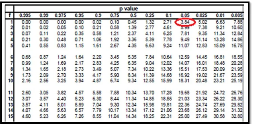
The portfolio with 9 exceptions (9 times the amount of portfolio’s daily returns/losses is greater that the estimated VaR calculation) is taken into consideration at the 90 % confidence level during the 251 trading/working days. First of all, the critical value is taken from the Critical Value χ² for the Chi-Squared Distribution (for 95 % confidence interval  critical value is 3.84):

Table 7. Chi-Squared Distribution

Source: Passel, 2016

The likelihood ratio test in this case equals to:

(10)

Test 2:

Furthermore, the portfolio with 10 exceptions (10 times the amount of portfolio’s daily returns/losses is greater that the estimated VaR calculation) is taken into consideration at the 95 % confidence interval during the 251 trading/working days. First of all, the critical value is taken from the Critical Value χ² for the Chi-Squared Distribution (for 95 % confidence interval  critical value is 3.84) same as in the previous example. The likelihood ratio test in this case equals to:

LR POF= 2ln =

Finally, for the third case the portfolio with 11 exceptions (11 times the amount of portfolio’s daily returns/losses is greater that the estimated VaR calculation) is taken into consideration at the 99% confidence interval during the 251 trading/working days. First of all, the critical value is taken from the Critical Value χ² for the Chi-Squared Distribution (for 95 % confidence interval  critical value is 3.84) same as in the previous two examples. The likelihood ratio test in this case equals to:

LR POF= -2ln =

Findings

The calculated likelihood ratio at 90 % and 99 % confidence level is in a great amount larger than the critical value. More precisely, since the calculated value 14.85 of likelihood test for the portfolio is greater than the critical value (p=1-c  p=1-0.95=0.05) 3.84; the statistic test shows that the model is rejected at the 90 % level of confidence. This means that the test outcome shows that the null hypothesis, which says that the model is “good“, is rejected with 90 % of confidence. The same is with the example for 99 % level of confidence: the calculated amount of LR is 15.82 and is greater than the critical value.

In other words, by calculating the likelihood ratio for levels 90 % and 99 % of confidence, it is identified that the observed rates of failure are different from the suggested by the confidence interval rate of failure. For these two tests (Test 1 and Test 3) it can be said as well that the VaR estimation underestimates the risk.

This is not the case with the portfolio at 95 %, where the calculated LR value is equal to 0.58 which is lower than the critical value. This indicates that the test outcome is to accept the model at 95 % of confidence.

The best overview of results is drawn in Table 7 which summarizes the calculated values for POF test at three confidence levels:

Table 7. POF test results

Confidence Level for Portfolio Test staticstics LR POF Critical value χ²(1) Test Outcome

90% 14.85 3.84 Reject

95% 0.58 3.84 Accept

99% 15.82 3.84 Reject

Kupiec's POF Test

LR

POF

= 0.58

(11)

Even though, by interpreting the results of Proportion of Failure test it is concluded that the model is not reliable at the 90 % and 99 % level of confidence, and that the rate of failure is different from the suggested rate by the confidence interval of failure, the results should always be confirmed with one more test (Haas, 2001) such as Kupiec TUFF Test or Christoffersen’s Independence Test.

4. Conclusion

It is well-know that the usage of VaR forecast is widespread. Since there is no such a method which predicts the accurate forecast, certain backtesting procedures should be undertaken in order to evaluate whether the calculated VaR results are satisfactory or not. Backtesting is definitely a necessity; however, more back tests should be done to confirm the accuracy and reliability of the VaR model validation. This fact indicates that the backtesting should be a part of daily VaR calculations. The results from backtesting are able to provide information whether potential problems or risks exist in the company's core system, so in that way the company’s management can take necessary risk mitigation measures and protect company against the potential future risk.

In this research using secondary data from http://finance.yahoo.com, daily share prices, daily returns for each company and daily returns of the entire portfolio of five companies during the period of 251 trading/working days are taken as crucial parameters. Test used for backtesting the forecasted VaR amount in this research is a so-called Proportion of Failure test. This test takes into account only the number of exceptions and not when the particular exception occurs. So, according to this fact, the number of exceptions is essential information necessary for further calculations and conclusions whether the model is accurate or not (should the null hypothesis be rejected or accepted).

The empirical example of Kupiec POF test presented in the research indicates that the model is rejected at the 90 % and 99 % confidence levels, since the calculated Test statistics LRPOF are greater than the critical value and that the model underestimates the risk (at the 90 % and 99 % confidence levels). However, not only one test is to be done: results from more tests should be analysed and compared in order to get an accurate conclusion whether potential problems are present in the model. Backtesting process should be the essential part of reporting regulation in every financial institution in order to be sure that the current VaR measure technique is ensuring consistent forecasts.

References

Brown, 2008 - Brown, A. (2008). Private Profits and Socialized Risk – Counterpoint: Capital Inadequacy, Global Association of Risk Professionals, 2008 cited by Reply in Definio Reply Backtesting, Available from: http://www.reply.eu/Documents/3036_img_DEFR09_ BackTesting_eng.pdf

Campbell, 2005 - Campbell, Sean D. (2005). A Review of Backtesting and Backtesting Procedures, 1st ed. 2005; Available from: https://www.federalreserve.gov/pubs/feds/2005/ 200521/200521pap.pdf [Accessed 14 April 2016].

Dowd, 1998 - Dowd, K. (1998). Beyond Value at Risk. The New Science of Risk Management, John Wiley & Sons, England.

Dowd, 2006 - Dowd, K. (2006). Retrospective Assessment of Value-at-Risk. Risk Management: A Modern Perspective, San Diego.

Emmer et al., 2015 - Emmer, S., Kratz, M., Tasche, D. (n.d) (2015). What is the Best Risk Measure in Practice? A Comparison of Standard Measures. Journal of Risk Model Validation. Available from: http://dx.doi.org/10.2139/ssrn.2370378 [Accessed 20 February 2016].

Graham, Pal, 2014 - Graham, A., Pal, J. (2014). Backtesting value-at-risk tail losses on a dynamic portfolio. Journal of Risk Model Validation. Available from: http://www.risk.net/journal- of-risk-model-validation/technical-paper/2350372/backtesting-value-at-risk-tail-losses-on-a-dynamic-portfolio [Accessed 20 January 2016].

(12)

Jorion, 2001 - Jorion, P. (2001). Value at Risk. The New Benchmark for Managing Financial Risk, 2nd Edition, McGraw-Hill, United States. Available from: https://www.scribd.com/doc/ 146088361/Value-at-Risk-3rd-Ed-the-New-Benchmark-for-Managing-Financial-Risk

Kupiec, 1995 - Kupiec, P. (1995). Techniques for Verifying the Accuracy of Risk Management Models, Journal of Derivatives; Available from: http://www.iijournals.com/doi/abs/10.3905/ jod.1995.407942?journalCode=jod

Passel, 2016 - Passel (2016). Plant and Soil Sciences e Library. Available at: http://passel.unl.edu/pages/informationmodule.php?idinformationmodule=1130447119&topicord er=8&maxto=16&minto=1 [Accessed 15 May. 2016].

Wiener, 1999 - Wiener, Z. (1999), Introduction to VaR (Value-at-Risk). Risk Management and Regulation in Banking, Kluwer Academic Publishers, Boston. Available from: http://pluto.mscc.huji.ac.il/~mswiener/research/Intro2VaR3.pdf