Plug-in Approach to Active Learning

Plug-in Approach to Active Learning

Stanislav Minsker SMINSKER@MATH.GATECH.EDU

686 Cherry Street School of Mathematics

Georgia Institute of Technology Atlanta, GA 30332-0160, USA

Editor: Sanjoy Dasgupta

Abstract

We present a new active learning algorithm based on nonparametric estimators of the regression function. Our investigation provides probabilistic bounds for the rates of convergence of the gen-eralization error achievable by proposed method over a broad class of underlying distributions. We also prove minimax lower bounds which show that the obtained rates are almost tight.

Keywords: active learning, selective sampling, model selection, classification, confidence bands

1. Introduction

Let(S,

B

)be a measurable space and let (X,Y)_∈S_{× {−}1,1_}be a random couple with unknown

distribution P. The marginal distribution of the design variable X will be denoted by Π. Let

η(x):=E(Y_|X =x) be the regression function. The goal of binary classification is to predict label Y based on the observation X . Prediction is based on a classifier - a measurable func-tion f : S_{7→ {−}1,1_}. The quality of a classifier is measured in terms of its generalization error, R(f) =Pr(Y₆= f(X)). In practice, the distribution P remains unknown but the learning algorithm has access to the training data - the i.i.d. sample(Xi,Yi),i=1. . .n from P. It often happens that the

cost of obtaining the training data is associated with labeling the observations Xiwhile the pool of

observations itself is almost unlimited. This suggests to measure the performance of a learning algo-rithm in terms of its label complexity, the number of labels Yirequired to obtain a classifier with the

desired accuracy. Active learning theory is mainly devoted to design and analysis of the algorithms that can take advantage of this modified framework. Most of these procedures can be characterized by the following property: at each step k, observation Xk is sampled from a distribution ˆΠkthat

de-pends on previously obtained(Xi,Yi), i≤k−1(while passive learners obtain all available training

data at the same time). ˆΠk is designed to be supported on a set where classification is difficult and

requires more labeled data to be collected. The situation when active learners outperform passive algorithms might occur when the so-called Tsybakov’s low noise assumption is satisfied: there exist constants B,γ>0 such that

∀t>0, Π(x :_|η(x)_{| ≤}t)_≤Btγ. (1)

This assumption provides a convenient way to characterize the noise level of the problem and will play a crucial role in our investigation.

generaliza-tion error of a resulting classifier can converge to zero exponentially fast with respect to its label complexity(while the best rate for passive learning is usually polynomial with respect to the cardi-nality of the training data set). However, available algorithms that adapt to the unknown parameters

of the problem(γin Tsybakov’s low noise assumption, regularity of the decision boundary) involve

empirical risk minimization with binary loss, along with other computationally hard problems, see Balcan et al. (2008), Dasgupta et al. (2008), Hanneke (2011) and Koltchinskii (2010). On the other hand, the algorithms that can be effectively implemented, as in Castro and Nowak (2008), are not adaptive.

The majority of the previous work in the field was done under standard complexity assumptions on the set of possible classifiers(such as polynomial growth of the covering numbers). Castro and Nowak (2008) derived their results under the regularity conditions on the decision boundary and the noise assumption which is slightly more restrictive then (1). Essentially, they proved that if the decision boundary is a graph of the H¨older smooth function g_∈Σ(β,K,[0,1]d−1_{)(see Section}

2 for definitions) and the noise assumption is satisfied withγ>0, then the minimax lower bound

for the expected excess risk of the active classifier is of order C_·N− β (1+γ)

2β+γ(d−1) _{and the upper bound is}

C(N/log N)−2ββ+(1γ(d+−γ)1)_{,where N is the label budget. However, the construction of the classifier that}

achieves an upper bound assumesβandγto be known.

In this paper, we consider the problem of active learning under classical nonparametric as-sumptions on the regression function - namely, we assume that it belongs to a certain H¨older class

Σ(β,K,[0,1]d_{)and satisfies to the low noise condition (1) with some positive} γ_{. In this case, the}

work of Audibert and Tsybakov (2005) showed that plug-in classifiers can attain optimal rates in the passive learning framework, namely, that the expected excess risk of a classifier ˆg=sign ˆηis

bounded above by C_·N−β

(1+γ)

2β+d _{(which is the optimal rate), where ˆ}η_{is the local polynomial estimator}

of the regression function and N is the size of the training data set. We were able to partially extend this claim to the case of active learning: first, we obtain minimax lower bounds for the excess risk of an active classifier in terms of its label complexity. Second, we propose a new algorithm that is based on plug-in classifiers, attains almost optimal rates over a broad class of distributions and possesses adaptivity with respect toβ,γ(within the certain range of these parameters).

The paper is organized as follows: the next section introduces remaining notations and specifies the main assumptions made throughout the paper. This is followed by a qualitative description of our learning algorithm. The second part of the work contains the statements and proofs of our main results - minimax upper and lower bounds for the excess risk.

2. Preliminaries

Our active learning framework is governed by the following rules:

1. Observations are sampled sequentially: Xk is sampled from the modified distribution ˆΠkthat

depends on(X1,Y1), . . . ,(Xk−1,Yk−1).

2. Yk is sampled from the conditional distribution PY|X(·|X =x). Labels are conditionally

inde-pendent given the feature vectors Xi,i≤n.

Usually, the distribution ˆΠkis supported on a set where classification is difficult.

Given the probability measure Q on S_{× {−}1,1_}, we denote the integral with respect to this

excess risk of f ∈

F

with respect to the measureQare defined by

RQ(f):=Q

I

y6=sign f(x)

E

Q(f):=RQ(f)−inf

g∈FRQ(g),

where

I

A is the indicator of event

A

. We will omit the subindexQwhen the underlying measure is

clear from the context. Recall that we denoted the distribution of(X,Y)by P. The minimal possible risk with respect to P is

R∗= inf

g:S7→[−1,1]Pr(Y 6=sign g(X)),

where the infimum is taken over all measurable functions. It is well known that it is attained for any g such that sign g(x) =signη(x)Π- a.s. Given g∈

F

, A∈

B

, δ>0, define

F

∞,A(g;δ):={f∈

F

: kf−gk∞,A≤δ},

where_kf₋g_k∞,A=sup x∈A|

f(x)₋g(x)_|. For A_∈

B

, define the function class

F

_|A:={f|A, f ∈

F

},

where f_|A(x):=f(x)

I

A(x). From now on, we restrict our attention to the case S= [0,1]d. Let K>0.

Definition 1 We say that g :Rd_7→Rbelongs toΣ(β,K,[0,1]d_{), the(β,K,[0,1]}d_{)- H¨older class of}

functions, if g is_⌊β_⌋times continuously differentiable and for all x,x1∈[0,1]dsatisfies

|g(x1)−Tx(x1)| ≤Kkx−x1kβ∞, where Tx is the Taylor polynomial of degree⌊β⌋of g at the point x.

Definition 2

P

(β,γ)is the class of probability distributions on[0,1]d_{×{−1,+1}with the following}

properties:

1. _∀t>0,Π(x :_|η(x)_{| ≤}t)_≤Btγ;

2. η(x)_∈Σ(β,K,[0,1]d_).

We do not mention the dependence of

P

(β,γ)on the fixed constants B,K explicitly, but this should not cause any uncertainty.

Finally, let us define

P

_U∗(β,γ)and

P

U(β,γ), the subclasses of

P

(β,γ), by imposing two additional

assumptions. Along with the formal descriptions of these assumptions, we shall try to provide some

motivation behind them. The first deals with the marginalΠ. For an integer M_≥1, let

G

M:=

k1 M, . . . ,

kd

M

, ki=1. . .M, i=1. . .d

be the regular grid on the unit cube[0,1]d _{with mesh size M}−1_{. It naturally defines a partition into}

a set of Md _{open cubes R}

i, i=1. . .Md with edges of length M−1 and vertices in

G

M. Below, we

Definition 3 We will say that Πis (u1,u2)-regular with respect to {

G

2m} if for any m≥1, any element of the partition Ri, i≤2dmsuch that Ri∩supp(Π)6=/0, we have

u1·2−dm≤Π(Ri)≤u2·2−dm, where 0<u1≤u2<∞.

Assumption 1 Πis(u1,u2)- regular.

In particular,(u1,u2)-regularity holds for the distribution with a density p on[0,1]d such that 0< u1≤p(x)≤u2<∞.

Let us mention that our definition of regularity is of rather technical nature; for most of the paper, the reader might think ofΠas being uniform on[0,1]d_{( however, we need slightly more complicated}

marginal to construct the minimax lower bounds for the excess risk). It is known that estimation of regression function in sup-norm is sensitive to the geometry of design distribution, mainly because the quality of estimation depends on the local amount of data at every point; conditions similar to our Assumption 1 were used in the previous works where this problem appeared, for example, strong density assumption in Audibert and Tsybakov (2005) and Assumption D in Ga¨ıffas (2007).

A useful characteristic of(u1,u2)- regular distributionΠis that this property is stable with re-spect to restrictions ofΠto certain subsets of its support. This fact fits the active learning framework particularly well.

Definition 4 We say thatQ belongs to

P

U(β,γ) if Q∈

P

(β,γ) and Assumption 1 is satisfied for

some u1,u2.

The second assumption is crucial in derivation of the upper bounds. The space of piecewise-constant functions which is used to construct the estimators ofη(x)is defined via

F

m=

(₂dm

∑

i=1

λiIRi(·): |λi| ≤1, i=1. . .2

dm

)

,

where_{R_i}2_i=1dm forms the dyadic partition of the unit cube. Note that

F

mcan be viewed as ak · k∞

-unit ball in the linear span of first 2dm Haar basis functions in[0,1]d_{. Moreover, {}

_F

m, m≥1}is

a nested family, which is a desirable property for the model selection procedures. By ¯ηm(x) we

denote the L2(Π)- projection of the regression function onto

F

m.

We will say that the set A_⊂[0,1]d _{approximates the decision boundary{x :}η_{(x) =0}if there}

exists t>0 such that

{x :_|η(x)_{| ≤}t_}Π⊆A_{Π⊆ {}x :_|η(x)_{| ≤}3t_}Π, (2)

where for any set A we define A_Π:=A_∩supp(Π). The most important example we have in mind

is the following: let ˆηbe some estimator ofηwith_kηˆ₋η_{k∞,supp(Π)≤}t,and define the 2t - band

aroundηby

ˆ

F=nf : ˆη(x)₋2t≤ f(x)_≤ηˆ(x) +2t ∀x∈[0,1]do_.

Take A=x : _∃f1,f2∈F s.t. sign fˆ 1(x)6=sign f2(x) , then it is easy to see that A satisfies (2). Modified design distributions used by our algorithm are supported on the sets with similar structure.

Assumption 2 There exists B2>0 such that for all m≥1, A∈σ(

F

m)satisfying (2) and such that

AΠ6=/0the following holds true:

Z

[0,1]d

(η₋η¯_m)2Π(dx_|x_∈A_Π)_≥B2kη−η¯mk2∞,AΠ.

Appearance of Assumption 2 is motivated by the structure of our learning algorithm - namely, it is based on adaptive confidence bands for the regression function. Nonparametric confidence bands is a big topic in statistical literature, and the review of this subject is not our goal. We just men-tion that it is impossible to construct adaptive confidence bands of optimal size over the whole

S

β≤1

Σ β,K,[0,1]d_{. Low (1997); Hoffmann and Nickl (to appear) discuss the subject in details.}

However, it is possible to construct adaptive L2 - confidence balls (see an example following

The-orem 6.1 in Koltchinskii, 2011). For functions satisfying Assumption 2, this fact allows to obtain confidence bands of desired size. In particular,

(a) functions that are differentiable, with gradient being bounded away from 0 in the vicinity of decision boundary;

(b) Lipschitz continuous functions that are convex in the vicinity of decision boundary

satisfy Assumption 2. For precise statements, see Propositions 15, 16 in Appendix A. A different approach to adaptive confidence bands in case of one-dimensional density estimation is presented in Gin´e and Nickl (2010). Finally, we define

P

U∗(β,γ):

Definition 5 We say thatQbelongs to

P

∗

U(β,γ)if Q∈

P

U(β,γ)and Assumption 2 is satisfied for

some B2>0.

2.1 Learning Algorithm

Now we give a brief description of the algorithm, since several definitions appear naturally in this

context. First, let us emphasize that the marginal distribution Πis assumed to be known to the

learner. This is not a restriction, since we are not limited in the use of unlabeled data andΠcan be estimated to any desired accuracy. Our construction is based on so-called plug-in classifiers of the form ˆf(_·) =sign ˆη(_·), where ˆηis a piecewise-constant estimator of the regression function. As we have already mentioned above, it was shown in Audibert and Tsybakov (2005) that in the passive

learning framework plug-in classifiers attain optimal rate for the excess risk of order N−β(

1+γ)

2β+d _{, with}

ˆ

ηbeing the local polynomial estimator.

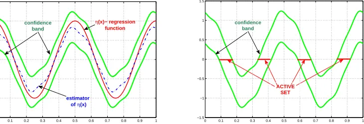
Our active learning algorithm iteratively improves the classifier by constructing shrinking

con-fidence bands for the regression function. On every step k, the piecewise-constant estimator ˆηk is

obtained via the model selection procedure which allows adaptation to the unknown smoothness(for H¨older exponent_≤1). The estimator is further used to construct a confidence band ˆ

F

kforη(x). The

active set associated with ˆ

F

kis defined as

ˆ

Ak=A(

F

ˆk):=

n

x_∈supp(Π): _∃f1,f2∈

F

ˆk,sign f1(x)6=sign f2(x)

o

.

requested only for observations X∈_Aˆ_{k, forcing the labeled data to concentrate in the domain where} higher precision is needed. This allows one to obtain a tighter confidence band for the regression function restricted to the active set. Since ˆAkapproaches the decision boundary, its size is controlled

by the low noise assumption. The algorithm does not require a priori knowledge of the noise and regularity parameters, being adaptive forγ>0,β_≤1. Further details are given in Section 3.2.

0 0.1 0.2 0.3 0.4 0.5 0.6 0.7 0.8 0.9 1 −1.5

−1 −0.5 0 0.5 1 1.5

confidence band

η(x)− regression function

estimator of η(x)

0 0.1 0.2 0.3 0.4 0.5 0.6 0.7 0.8 0.9 1 −1.5

−1 −0.5 0 0.5 1 1.5

confidence band

ACTIVE SET

Figure 1: Active Learning Algorithm

2.2 Comparison Inequalities

Before proceeding with the main results, let us recall the well-known connections between the binary risk and the_{k · k∞},_{k · kL2(Π)}- norm risks:

Proposition 6 Under the low noise assumption,

RP(f)−R∗≤D1k(f−η)

I

{sign f 6=signη}k1+_∞ γ; (3)

RP(f)−R∗≤D2k(f−η)

I

{sign f 6=signη}k

2(1+γ)

2+γ

L2(Π); (4)

RP(f)−R∗≥D3Π(sign f 6=signη)

1+γ

γ _{. (5)}

Proof For (3) and (4), see Audibert and Tsybakov (2005), Lemmas 5.1 and 5.2 respectively, and for (5)—Koltchinskii (2011), Lemma 5.2.

3. Main Results

The question we address below is: what are the best possible rates that can be achieved by active algorithms in our framework and how these rates can be attained.

3.1 Minimax Lower Bounds For the Excess Risk

The goal of this section is to prove that for P_∈

P

(β,γ), no active learner can output a classifier with

expected excess risk converging to zero faster than N− β

(1+γ)

2β+d−βγ_{. Our result builds upon the minimax}

Remark The theorem below is proved for a smaller class

P

∗

U(β,γ), which implies the result for

P

(β,γ).

Theorem 7 Letβ,γ,d be such thatβγ_≤d. Then there exists C>0 such that for all n large enough and for any active classifier ˆfn(x)we have

sup

P∈P∗

U(β,γ)

ERP(fˆn)−R∗≥CN− β(1+γ)

2β+d−βγ_.

Proof We proceed by constructing the appropriate family of classifiers fσ(x) =signησ(x), in a way similar to Theorem 3.5 in Audibert and Tsybakov (2005), and then apply Theorem 2.5 from Tsybakov (2009). We present it below for reader’s convenience.

Theorem 8 Let Σbe a class of models, d :Σ_×Σ_7→R- the pseudometric and Pf, f ∈Σ - a

collection of probability measures associated withΣ. Assume there exists a subset_{f0, . . . ,fM}ofΣ

such that

1. d(fi,fj)≥2s>0 for all 0≤i< j≤M;

2. Pfj ≪Pf0 for every 1≤ j≤M;

3. _M1

M

∑

j=1

KL(Pfj,Pf0)≤αlog M, 0<α< 1 8. Then

inf ˆ

f

sup

f_∈Σ

Pf d(fˆ,f)≥s

≥ √

M

1+√M 1−2α−

s

2α log M

!

,

where the infimum is taken over all possible estimators of f based on a sample from Pf and KL(·,·)

is the Kullback-Leibler divergence.

Going back to the proof, let q=2l,l_≥1 and

Gq:=

2k1₋1

2q , . . . ,

2kd−1

2q

,ki=1. . .q,i=1. . .d

be the grid on[0,1]d_{. For x∈[0,1]}d_{, let}

nq(x) =argmin kx−xkk2: xk∈Gq .

If nq(x)is not unique, we choose a representative with the smallest k · k2 norm. The unit cube is partitioned with respect to Gq as follows: x1,x2 belong to the same subset if nq(x1) =nq(x2). Let

′_≻′ _{be some order on the elements of Gq such that x≻y implieskxk2≥ kyk2. Assume that the}

elements of the partition are enumerated with respect to the order of their centers induced by′_≻′:

[0,1]d₌ q

d

S

i=1

Ri. Fix 1≤m≤qdand let

S :=

m

[

Note that the partition is ordered in such a way that there always exists 1≤k≤q√d with

B+

0,k q

⊆S_⊆B+ 0,k+3

√

d q

!

, (6)

where B+(0,R):=x∈Rd+: kxk2≤R . In other words, (6) means that that the difference between the radii of inscribed and circumscribed spherical sectors of S is of order C(d)q−1.

Let v>r1>r2be three integers satisfying

2−v<2−r1<2−r1√d<2−r2√d<2−1. (7)

Define u(x):R_7→R₊by

u(x):=

R_∞

x U(t)dt

1/2_R 2−v

U(t)dt

, (8)

where

U(t):=

(

exp

− 1

(1/2−x)(x₋2−v₎

, x∈(2−v_,1 2)

0 else.

Note that u(x) is an infinitely differentiable function such that u(x) =1, x_∈[0,2−v]and u(x) = 0, x_≥1₂. Finally, for x_∈Rdlet

Φ(x):=Cu(_kx_k2),

where C :=CL,βis chosen such thatΦ∈Σ(β,L,Rd). Let rS:=inf{r>0 : B+(0,r)⊇S}and

A0:=

(

[

i

Ri: Ri∩B+

0,rS+q− βγ

d

= /0

)

.

Note that

rS≤c

m1/d

q , (9)

since Vol(S) =mq−d.

Define

H

m={Pσ:σ∈ {−1,1}m}to be the hypercube of probability distributions on[0,1]d× {−1,+1_}. The marginal distributionΠof X is independent ofσ: define its density p by

p(x) =

    

2d(r1−1)

2d(r1−r2)₋₁, x∈B∞

z,2−r2

q

\B_∞z,2−r1

q

, z_∈Gq∩S,

c0, x∈A0,

0 else.

where B∞(z,r):=_{x : _kx₋z_k∞≤r_}, c0:= 1_Vol(−mq_A0−₎d(note thatΠ(Ri) =q−d ∀i≤m) and r1,r2are

defined in (7). In particular,Πsatisfies Assumption 1 since it is supported on the union of dyadic

cubes and has bounded above and below on supp(Π)density. Let

Ψ(x):=u1/2₋qβγddist2(_x,_B+(0,_rS))

Figure 2: Geometry of the support

where u(_·)is defined in (8) and dist2(x,A):=inf{kx−yk2,y∈A}. Finally, the regression functionη_σ(x) =E_Pσ(Y_|X=x)is defined via

ησ(x):=

( _σ

iq−βΦ(q[x−nq(x)]), x∈Ri, 1≤i≤m

1

CL,β

√

ddist2(x,B+(0,rS))

d

γ_·Ψ_{(x), x∈[0,1]}d_\S.

The graph ofη_σ is a surface consisting of small ”bumps” spread around S and tending away from

0 monotonically with respect to dist2(·,B+(0,rS))on[0,1]d\S. Clearly,ησ(x)satisfies smoothness

requirement,1since for x_∈[0,1]d

dist2(x,B+(0,rS)) = (kxk2−rS)∨0.

Let’s check that it also satisfies the low noise condition. Since_|η_{σ| ≥}Cq−βon the support ofΠ, it is enough to consider t=Czq−βfor z>1:

Π(_|ησ(x)_{| ≤}Czq−β)_≤mq−d+Πdist2(x,B+(0,rS))≤Czγ/dq− βγ

d

≤

≤mq−d+C2

rS+Czγ/dq− βγ

d

d ≤

≤mq−d+C3mq−d+C4zγq−βγ≤

≤Ctbγ,

if mq−d=O(q−βγ). Here, the first inequality follows from consideringησon S and A0 separately, and second inequality follows from (9) and direct computation of the sphere volume.

Finally,η_σsatisfies Assumption 2 with some B2:=B2(q)since on supp(Π) 0<c1(q)_{≤ k}∇ησ(x)_k2≤c2(q)<∞.

The next step in the proof is to choose the subset of

H

which is “well-separated”: this can be done

due to the following fact (see Tsybakov, 2009, Lemma 2.9):

Proposition 9 (Gilbert-Varshamov) For m≥8, there exists

{σ0, . . . ,σM} ⊂ {−1,1}m

such thatσ0={1,1, . . . ,1},ρ(σi,σj)≥ m₈ ∀0≤i<k≤M and M≥2m/8 whereρstands for the

Hamming distance.

Let

H

′_:={Pσ

0, . . . ,PσM} be chosen such that{σ0, . . . ,σM} satisfies the proposition above. Next, following the proof of Theorems 1 and 3 in Castro and Nowak (2008), we note that_∀σ_∈

H

′,σ₆=σ0

KL(P_σ,NkPσ0,N)≤8N max

x∈[0,1](ησ(x)−ησ0(x)) 2

≤32C_L2_,βNq−2β, (10)

where P_σ,N is the joint distribution of (Xi,Yi)Ni=1 under hypothesis that the distribution of couple (X,Y)is Pσ. Let us briefly sketch the derivation of (10); see also the proof of Theorem 1 in Castro and Nowak (2008). Denote

¯

Xk:= (X1, . . . ,Xk),

¯

Yk := (Y1, . . . ,Yk).

Then dP_σ,Nadmits the following factorization:

dP_σ,N(X¯N,Y¯N) = N

∏

i=1

P_σ(Y_i|Xi)dP(Xi|X¯i−1,Y¯i−1),

where dP(Xi|X¯i₋1,Y¯i₋1) does not depend onσ but only on the active learning algorithm. As a

consequence,

KL(P_σ,NkPσ0,N) =EPσ,Nlog

dP_σ,N(X¯N,Y¯N)

dPσ0,N(X¯n,Y¯N)

=E_Pσ,Nlog ∏

N

i=1Pσ(Yi|Xi)

∏N

i=1Pσ0(Yi|Xi)

=

=

N

∑

i=1

E_Pσ,N

E_Pσ

log Pσ(Yi|Xi) P_σ0(Y_i|Xi)|

Xi

≤

≤N max

x∈[0,1]d

E_Pσ

log Pσ(Y1|X1) Pσ0(Y1|X1)

|X1=x

≤

≤8N max

x∈[0,1]d(ησ(x)−ησ0(x)) 2_,

where the last inequality follows from Lemma 1 (Castro and Nowak, 2008). Also, note that we have max_x∈[0,1]d in our bounds rather than the average over x that would appear in the passive learning framework.

It remains to choose q,m in appropriate way: set q=_⌊C1N

1

2β+d−βγ_{⌋and m=⌊C2q}d₋βγ_⌋where

C1, C2 are such that qd ≥m≥1 and 32C2_L,βNq−2β< ₆₄m which is possible for N big enough. In particular, mq−d=O(q−βγ). Together with the bound (10), this gives

1 M_σ

∑

∈H′

KL(PσkP_σ0)≤32C_u2Nq−2β<

m 82 =

1 8log|

H

so that conditions of Theorem 8 are satisfied. Setting

fσ(x):=signησ(x),

we finally have_∀σ16=σ2∈

H

′

d(f_σ1,f_σ2):=Π(signη_σ1(x)₆=signη_σ2(x))_≥ m

8qd ≥C4N

−_2β+dβγ−βγ_,

where the lower bound just follows by construction of our hypotheses. Since under the low noise assumption RP(fˆn)−R∗≥cΠ(fˆn6=signη)

1+γ

γ _{(see (5)), we conclude by Theorem 8 that}

inf ˆ

fN sup

P∈P∗

U(β,γ) Pr

RP(fˆn)−R∗≥C4N−

β(1+γ)

2β+d−βγ

≥

≥inf

ˆ

fN sup

P∈P∗

U(β,γ) Pr

Π(fˆn(x)6=signηP(x))≥

C4

2 N

−2β+dβγ−βγ

≥τ>0.

3.2 Upper Bounds For the Excess Risk

Below, we present a new active learning algorithm which is computationally tractable, adaptive with respect toβ,γ( in a certain range of these parameters) and can be applied in the nonparametric setting. We show that the classifier constructed by the algorithm attains the rates of Theorem 7, up to polylogarithmic factor, if 0<β_≤1 andβγ_≤d (the last condition covers the most interesting case when the regression function hits or crosses the decision boundary in the interior of the support ofΠ; for detailed statement about the connection between the behavior of the regression function near the

decision boundary with parametersβ, γ, see Proposition 3.4 in Audibert and Tsybakov, 2005). The

problem of adaptation to higher order of smoothness (β>1) is still awaiting its complete solution; we address these questions below in our final remarks.

For the purpose of this section, the regularity assumption reads as follows: there exists 0<β_≤1 such that_∀x1,x2∈[0,1]d

|η(x1)−η(x2)| ≤B1kx1−x2kβ_∞. (11)

Since we want to be able to construct non-asymptotic confidence bands, some estimates on the size of constants in (11) and Assumption 2 are needed. Below, we will additionally assume that

B1≤log N, B2≥log−1N,

where N is the label budget. This can be replaced by any known bounds on B1,B2.

Let A_∈σ(

F

m)with AΠ:=A∩supp(Π)6=/0. Define

ˆ

and dm:=dim

F

m|AΠ. Next, we introduce a simple estimator of the regression function on the set

AΠ. Given the resolution level m and an iid sample(Xi,Yi),i≤N with Xi∼ΠˆA, let

ˆ

ηm,A(x):=

∑

i:Ri∩AΠ6=/0

∑N

j=1Yj

I

Ri(Xj)

N·_Πˆ_A(Ri)

I

Ri(x). (12)

Since we assumed that the marginal Π is known, the estimator is well-defined. The following

proposition provides the information about concentration of ˆηmaround its mean:

Proposition 10 For all t>0,

Pr max

x∈AΠ|

ˆ

ηm,A(x)−η¯m(x)| ≥t

s

2dmΠ_(A)

u1N

!

≤

≤2dmexp −

t2 2(1+₃tp2dmΠ_(A)/u

1N)

!

,

Proof This is a straightforward application of the Bernstein’s inequality to the random variables

Si_N:=

N

∑

j=1

Yj

I

Ri(Xj),i∈ {i : Ri∩AΠ6= /0},

and the union bound: indeed, note thatE(Y

I

Ri(Xj)) 2₌Π_ˆ

A(Ri), so that

PrSi_N−N

Z

Ri

ηd ˆΠA

≥tN ˆΠA(Ri)

≤2 exp

−N ˆΠA(Ri)t

2 2+2t/3

,

and the rest follows by simple algebra using that ˆΠA(Ri)≥₂dmu1_Π(A) by the(u1,u2)-regularity ofΠ.

Given a sequence of hypotheses classes

G

m,m≥1, define the index set

J

(N):=

m∈N: 1≤dim

G

m≤

N log2N

(13)

- the set of possible “resolution levels” of an estimator based on N classified observations(an upper bound corresponds to the fact that we want the estimator to be consistent). When talking about model selection procedures below, we will implicitly assume that the model index is chosen from

the corresponding set

J

. The role of

G

mwill be played by

F

m|Afor appropriately chosen set A. We

are now ready to present the active learning algorithm followed by its detailed analysis(see Table 1).

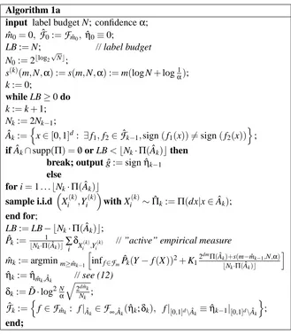
Remark Note that on every iteration, Algorithm 1a uses the whole sample to select the resolu-tion level ˆmk and to build the estimator ˆηk. While being suitable for practical implementation, this

is not convenient for theoretical analysis. We will prove the upper bounds for a slighly modified version: namely, on every iteration k labeled data is divided into two subsamples Sk,1 and Sk,2 of approximately equal size,_|Sk,1| ≃ |Sk,2| ≃1₂Nk·Π(Aˆk). Then S1,k is used to select the resolution

Algorithm 1a

input label budget N; confidenceα; ˆ

m0=0,

F

ˆ0:=

F

m0ˆ ,ηˆ0≡0;

LB :=N; // label budget

N0:=2⌊log2

√

N⌋_;

s(k)(m,N,α):=s(m,N,α):=m(log N+log_α1); k :=0;

while LB_≥0 do k :=k+1; Nk:=2Nk−1;

ˆ Ak:=

n

x_∈[0,1]d_{: ∃f}

1,f2∈

F

ˆk−1,sign(f1(x))6=sign(f2(x))

o

;

if ˆAk∩supp(Π) =/0or LB<⌊Nk·Π(Aˆk)⌋then

break; output ˆg :=sign ˆηk₋1 else

for i=1. . ._⌊Nk·Π(Aˆk)⌋

sample i.i.d X_i(k),Y_i(k)with X_i(k)_∼Πˆk:=Π(dx|x∈Aˆk);

end for;

LB :=LB_{− ⌊}Nk·Π(Aˆk)⌋;

ˆ

Pk:= 1

⌊Nk·Π(Aˆk)⌋∑_i δXi(k),Y (k) i

// ”active” empirical measure

ˆ

mk:=argminm≥mˆk−1

h

inff∈FmPˆk(Y−f(X)) 2_+K

12 dm_Π(Aˆ

k)+s(m−mˆk−1,N,α)

⌊Nk·Π(Aˆk)⌋

i

ˆ

ηk:=ηˆ_mˆk,Aˆ_k // see (12)

δk:=D˜·log2 N_α

q

2d ˆ_mk

Nk ; ˆ

F

k:=

n

f _∈

F

mˆk : f|Aˆk ∈

F

∞,Aˆk(ηˆk;δk), f|[0,1]d\Aˆk ≡ηˆk−1|[0,1]d\Aˆk

o

;

end;

Table 1: Active Learning Algorithm

As a first step towards the analysis of Algorithm 1b, let us prove the useful fact about the general model selection scheme. Given an iid sample(Xi,Yi),i≤N, set sm=m(s+log log2N),m≥1 and

ˆ

m :=mˆ(s) =argmin_m∈J(N)

inf

f∈Fm

PN(Y−f(X))2+K1

2dm+sm

N

,

¯

m :=min

m≥1 : inf

f∈Fm

E(f(X)₋η(X))2_≤K 2

2dm

N

.

Theorem 11 There exist an absolute constant K1big enough such that, with probability_≥1₋e−s,

ˆ m_≤m¯.

Proof See Appendix B.

Corollary 12 Supposeη(x)_∈Σ(β,L,[0,1]d_{). Then, with probability≥1−e}−s_,

2mˆ _≤C1·N

1 2β+d

Proof By definition of ¯m, we have

¯

m_≤1+max

m : inf

f∈Fm

E(f(X)₋η(X))2>K2 2dm

N

≤

≤1+max

m : L22−2βm>K2 2dm

N

,

and the claim follows.

With this bound in hand, we are ready to formulate and prove the main result of this section:

Theorem 13 Suppose that P_∈

P

∗

U(β,γ) with B1≤log N, B2≥log−1N and βγ≤d. Then, with probability_≥1₋3α, the classifier ˆg returned by Algorithm 1b with label budget N satisfies

RP(gˆ)−R∗≤Const·N− β(1+γ)

2β+d−βγ_logpN

α,

where p_≤22_ββγ₊(1+_d−βγγ) and B1, B2are the constants from (11) and Assumption 2. Remarks

1. Note that when βγ> d

3, N

−_2ββ+d(1+−γ)βγ _{is a fast rate, that is, faster than N}−1

2; at the same time,

the passive learning rate N−

β(1+γ)

2β+d _{is guaranteed to be fast only when}βγ_>d

2, see Audibert and Tsybakov (2005).

2. For ˆα_≃N− β (1+γ)

2β+d−βγ _{Algorithm 1b returns a classifier ˆgαˆ that satisfies}

ERP(gˆαˆ)−R∗≤Const·N−

β(1+γ)

2β+d−βγ_logp_N.

This is a direct corollary of Theorem 13 and the inequality

E_|Z_{| ≤}t+_kZ_k∞Pr(_|Z_{| ≥}t).

Proof Our main goal is to construct high probability bounds for the size of the active sets defined

by Algorithm 1b. In turn, these bounds depend on the size of the confidence bands forη(x), and

the previous result(Theorem 11) is used to obtain the required estimates. Suppose L is the number

of steps performed by the algorithm before termination; clearly, L_≤N.

Let N_kact:=_⌊Nk·Π(Aˆk)⌋be the number of labels requested on k-th step of the algorithm: this

choice guarantees that the ”density” of labeled examples doubles on every step.

Claim: the following bound for the size of the active set holds uniformly for all 2_≤k_≤L with

probability at least 1₋2α:

Π(_Aˆ_k)≤CN−2ββγ+d

k

logN_α

2γ

It is not hard to finish the proof assuming (14) is true: indeed, it implies that the number of labels requested on step k satisfies

N_kact=_⌊NkΠ(Aˆk)⌋ ≤C·N 2β+d−βγ

2β+d

k

logN

α

2γ

with probability_≥1₋2α. Since∑

k

N_kact_≤N, one easily deduces that on the last iteration L we have

NL≥c

N log2γ(N/α)

2β+d

2β+d−βγ

(15)

To obtain the risk bound of the theorem from here, we apply2inequality (3) from Proposition 6:

RP(gˆ)−R∗≤D1k(ηˆL−η)·

I

{sign ˆηL=6 signη}k1+_∞ γ. (16)

It remains to estimatekηˆL−ηk_∞,Aˆ_L: we will show below while proving (14) that

kηˆL−ηk_∞,AˆL≤C·N

−2ββ+d

L log2

N

α.

Together with (15) and (16), it implies the final result.

To finish the proof, it remains to establish (14). Recall that ¯ηkstands for the L2(Π)- projection

ofηonto

F

mˆk. An important role in the argument is played by the bound on the L2(Πˆk)- norm of the “bias”(η¯_k−η): together with Assumption 2, it allows to estimate_kη¯_k−η_k∞,Aˆ

k. The required

bound follows from the following oracle inequality: there exists an event

B

of probability_≥1₋α

such that on this event for every 1_≤k_≤L

kη¯_k−η_k2

L2(_Πˆ_k)≤ inf

m≥mˆk−1

"

inf

f_∈Fmk

f₋η_k2_L2(Πˆ

k)+ (17)

+K1

2dmΠ(_Aˆ_{k) + (m−mˆk−1)log(N/α)} NkΠ(Aˆk)

#

.

It general form, this inequality is given by Theorem 6.1 in Koltchinskii (2011) and provides the estimate for _kηˆk−ηkL2_(Πˆ_k), so it automatically implies the weaker bound for the bias term only. To deduce (17), we use the mentioned general inequality L times(once for every iteration) and the union bound. The quantity 2dmΠ(Aˆk) in (17) plays the role of the dimension, which is justified

below. Let k_≥1 be fixed. For m_≥mˆk−1, consider hypothesis classes

F

m|_Aˆ_k:=

n

f

I

_Aˆ_k, f ∈

F

m

o

.

An obvious but important fact is that for P_∈

P

U(β,γ), the dimension of

F

m|Aˆk is bounded by u

−1 1 · 2mΠ(_Aˆ_{k): indeed,}

Π(_Aˆ_{k) =}

∑

j:Rj∩Aˆk6=/0

Π(Rj)≥u12−dm·#

j : Rj∩Aˆk6=/0 ,

hence

dim

F

m|_Aˆ_k=#j : Rj∩Aˆk=6 /0 ≤u−₁1·2mΠ(Aˆk). (18)

Theorem 11 applies conditionally on nX_i(j)oNj

i=1, j≤k−1 with sample of size N

act

k and s=

log(N/α): to apply the theorem, note that, by definition of ˆAk, it is independent of Xi(k),i=1. . .Nkact.

Arguing as in Corollary 12 and using (18), we conclude that the following inequality holds with probability_≥1₋α_N for every fixed k:

2mˆk_≤C·N

1 2β+d

k . (19)

Let

E

1be an event of probability≥1−αsuch that on this event bound (19) holds for every step k,

k_≤L and let

E

2be an event of probability≥1−αon which inequalities (17) are satisfied. Suppose

that event

E

1∩

E

2 occurs and let k0 be a fixed arbitrary integer 2≤k0≤L+1. It is enough to

assume that ˆAk0−1is nonempty(otherwise, the bound trivially holds), so that it contains at least one cube with sidelength 2−mˆk0−2 _and

Π(Aˆk0−1)≥u12−d ˆmk0−1≥cN−

d

2β+d

k0 . (20)

Consider inequality (17) with k=k0−1 and 2m≃N

1 2β+d

k0−1. By (20), we have

kη¯k0₋1−ηk_L22 _(Πˆ_k0−1)≤CN

−2β2β+d

k0−1 log 2N

α. (21)

For convenience and brevity, denoteΩ:=supp(Π). Now Assumption 2 comes into play: it implies,

together with (21) that

CN−

β 2β+d

k0−1 log N

α ≥ kη¯k0−1−ηkL2_(Πˆ

k0−1)≥B2kη¯k0−1−ηk∞,Ω∩Aˆ_k0−1. (22)

To bound

kηˆk0₋1(x)−η¯k0₋1(x)k_∞,Ω∩Aˆ k0−1

we apply Proposition 10. Recall that ˆmk0−1depends only on the subsample Sk0−1,1but not on Sk0−1,2. Let

T

k:=

n

X_i(j),Y_i(j)oN

act

j

i=1, j≤k−1

∪Sk,1

be the random vector that defines ˆAkand resolution level ˆmk. Note that for any x,

E(ηˆk0−1(x)|

T

k0−1)a.s.=η¯mˆ_k0−1(x).

Proposition 10 thus implies

Pr max

x∈Ω∩Aˆ_k0−1

|ηˆk0−1(x)−η¯mˆ_k0−1(x)| ≥Kt

s

2d ˆmk0−1

Nk0₋1

T

k0−1

!

≤

≤N exp

−t2

2(1+t

3C3)

Choosing t=c log(N/α)and taking expectation, the inequality(now unconditional) becomes

Pr

  max

x∈Ω∩_Aˆ k0−1

|ηˆmˆ_k0−1(x)−η¯mˆ_k0−1(x)| ≤K

s

2d ˆmk0−1_log2_(N/α₎

Nk0−1



_≥1₋α. (23)

Let

E

3be the event on which (23) holds true. Combined, the estimates (19),(22) and (23) imply that

on

E

1∩

E

2∩

E

3

kη−ηˆk0−1k_∞,Ω∩Aˆ

k0−1 ≤ kη−η¯k0−1k∞,Ω∩Aˆ_k0−1+kη¯k0−1−ηˆk0−1k∞,Ω∩Aˆ_k0−1

≤ C

B2 N−

β 2β+d

k0−1 log N

α+K

s

2d ˆmk0−1_log2_(N/α₎

Nk0−1 ≤

(24)

≤(K+C)_·N−

β 2β+d

k0−1 log 2N

α,

where we used the assumption B2≥log−1N. Now the width of the confidence band is defined via

δk:=2(K+C)·N

−2ββ+d

k0−1 log 2N

α (25)

(in particular, ˜D from Algorithm 1a is equal to 2(K+C)). With the bound (24) available, it is

straightforward to finish the proof of the claim. Indeed, by (25) and the definition of the active set, the necessary condition for x_∈Ω_∩Aˆk0 is

|η(x)_{| ≤}3(K+C)_·N−

β 2β+d

k0−1 log 2N

α,

so that

Π(Aˆk0) =Π(Ω∩Aˆk0)≤Π

|η(x)_{| ≤}3(K+C)_·N−

β 2β+d

k0−1 log 2N

α

≤

≤_BN˜ −

βγ 2β+d

k0−1 log 2γN

α.

by the low noise assumption. This completes the proof of the claim since Pr(

E

1∩

E

2∩

E

3)≥

1₋3α.

We conclude this section by discussing running time of the active learning algorithm. Assume that the algorithm has access to the sampling subroutine that, given A_⊂[0,1]d_{withΠ(A)>0, generates}

i.i.d.(Xi,Yi)with Xi∼Π(dx|x∈A).

Proposition 14 The running time of Algorithm 1a(1b) with label budget N is

O

(dN log2N).

Remark In view of Theorem 13, the running time required to output a classifier ˆg such that RP(gˆ)−

R∗_≤εwith probability_≥1₋αis

O

 

1

ε

2β+d−βγ

β(1+γ) poly

log 1

εα

Proof We will use the notations of Theorem 13. Let N_kact be the number of labels requested by the algorithm on step k. The resolution level ˆmk is always chosen such that ˆAk is partitioned into

at most N_kact dyadic cubes, see (13). This means that the estimator ˆηk takes at most Nkact distinct

values. The key observation is that for any k, the active set ˆAk+1is always represented as the union of a finite number(at most N_kact) of dyadic cubes: to determine if a cube Rj⊂Aˆk+1, it is enough to

take a point x_∈Rjand compare sign(ηˆk(x)−δk)with sign(ηˆk(x) +δk): Rj∈Aˆk+1only if the signs are different(so that the confidence band crosses zero level). This can be done in

O

(Nact

k )steps.

Next, resolution level ˆmkcan be found in

O

(N_kactlog2N)steps: there are at most log2Nkactmodels

to consider; for each m, inff∈FmPˆk(Y−f(X))

2_{is found explicitly and is achieved for the} piecewise-constant ˆf(x) = ∑iY

(k) i IR j(Xi(k))

∑iIR j(Xi(k))

, x_∈Rj.Sorting of the data required for this computation is done in

O

(dN_kactlog N)steps for each m, so the whole k-th iteration running time is

O

(dN_kactlog2N). Since

∑

k

N_kact_≤N, the result follows.

4. Conclusion and Open Problems

We have shown that active learning can significantly improve the quality of a classifier over the passive algorithm for a large class of underlying distributions. Presented method achieves fast rates of convergence for the excess risk, moreover, it is adaptive(in the certain range of smoothness and

noise parameters) and involves minimization only with respect to quadratic loss(rather than the 0₋1

loss).

The natural question related to our results is:

• Can we implement adaptive smooth estimators in the learning algorithm to extend our results

beyond the caseβ_≤1?

The answer to this second question is so far an open problem. Our conjecture is that the correct

rate of convergence for the excess risk is, up to logarithmic factors, N− β

(1+γ)

2β+d−γ(β∧1)_{,which coincides}

with presented results forβ_≤1. This rate can be derived from an argument similar to the proof of

Theorem 13 under the assumption that on every step k one could construct an estimator ˆηk with

kη−ηˆ_kk∞,Aˆ_k.N

−2ββ+d

k .

At the same time, the active set associated to ˆηk should maintain some structure which is suitable

for the iterative nature of the algorithm. Transforming these ideas into a rigorous proof is a goal of our future work.

Acknowledgments

I want to express my sincere gratitude to my Ph.D. advisor, Dr. Vladimir Koltchinskii, for his support and numerous helpful discussions.

I am grateful to the anonymous reviewers for carefully reading the manuscript. Their insightful and wise suggestions helped to improve the quality of presentation and results.

Appendix A. Functions Satisfying Assumption 2

In the propositions below, we will assume for simplicity that the marginal distributionΠis

abso-lutely continuous with respect to Lebesgue measure with density p(x)such that

0<p1≤p(x)≤p2<∞for all x∈[0,1]d. Given t_∈(0,1], define At :={x : |η(x)| ≤t}.

Proposition 15 Supposeηis Lipschitz continuous with Lipschitz constant S. Assume also that for some t_∗>0 we have

(a) Π At_∗/3

>0;

(b) ηis twice differentiable for all x_∈At_∗;

(c) infx∈At_∗k∇η(x)k1≥s>0; (d) sup_x∈At

∗kD

2η_{(x)k ≤C<}∞_{wherek · kis the operator norm.} Thenηsatisfies Assumption 2.

Proof By intermediate value theorem, for any cube Ri, 1≤i≤2dm there exists x0∈Ri such that

¯

ηm(x) =η(x0),x∈Ri. This implies

|η(x)₋η¯_m(x)_|=_|η(x)₋η(x0)|=|∇η(ξ)·(x−x0)| ≤

≤ k∇η(ξ)_k1kx−x0k∞≤S·2−m. On the other hand, if Ri⊂At∗ then

|η(x)₋η¯_m(x)_|=_|η(x)₋η(x0)|= =_|∇η(x0)·(x−x0) +

1 2[D

2_{η(ξ)](x−x}

0)·(x−x0)| ≥

≥ |∇η(x0)_·(x₋x0)_{| −}1 2sup_ξ kD

2_η(ξ)

kmax

x_∈Rik

x₋x0k22≥ (26)

≥ |∇η(x0)·(x−x0)| −C12−2m. Note that a strictly positive continuous function

h(y,u) =

Z

[0,1]d

(u_·(x₋y))2dx

achieves its minimal value h_∗>0 on a compact set[0,1]d_×u∈Rd_:kuk

1=1 . This implies(using

(26) and the inequality(a₋b)2_≥ a2

2 −b 2₎

Π−1_(R

i)

Z

Ri

(η(x)₋η¯m(x))2p(x)dx≥

≥1₂(p22dm)−1

Z

Ri

(∇η(x0)·(x−x0))2p1dx−C122−4m≥

≥1

2 p1 p2k

Now take a set A∈σ(

F

m), m≥m0from Assumption 2. There are 2 possibilities: either A⊂At∗ or

A_⊃At∗/3. In the first case the computation above implies

Z

[0,1]d

(η₋η¯m)2Π(dx|x∈A)≥c22−2m= c2 S2S

2₂−2m_≥

≥_Sc22kη−η¯mk 2 ∞,A.

If the second case occurs, note that, sincex : 0<_|η(x)_|<t∗

3 has nonempty interior, it must

con-tain a dyadic cube R_∗with edge length 2−m∗_{. Then for any m≥max(m0,m}

∗) Z

[0,1]d

(η₋η¯_m)2Π(dx_|x_∈A)_≥

≥Π−1(A)

Z

R∗

(η₋η¯m)2Π(dx)≥

c2

42

−2m_Π(R

∗)≥

≥c_S2₂Π(R_∗)_kη₋η¯_mk2_∞,A and the claim follows.

The next proposition describes conditions which allow functions to have vanishing gradient on decision boundary but requires convexity and regular behaviour of the gradient.

Everywhere below,∇ηdenotes the subgradient of a convex functionη.

For 0<t1<t2, define G(t1,t2):= sup x∈_At2\_At1k

∇η(x)k1

inf

x∈_At2\_At1k∇η(x)k1

. In case when∇η(x)is not unique, we choose

a representative that makes G(t1,t2)as small as possible.

Proposition 16 Supposeη(x)is Lipschitz continuous with Lipschitz constant S. Moreover, assume that there exists t_∗>0 and q :(0,∞)_7→(0,∞)such that At_∗ ⊂ (0,1)dand

(a) b1tγ≤Π(At)≤b2tγ∀t<t∗;

(b) For all 0<t1<t2≤t∗,G(t1,t2)≤q

t2 t1

;

(c) Restriction ofηto any convex subset of At∗ is convex.

Thenηsatisfies Assumption 2.

Remark The statement remains valid if we replaceηby_|η_|in (c).

Proof Assume that for some t_≤t_∗and k>0

R_⊂At\At/k

is a dyadic cube with edge length 2−m and let x0 be such that ¯ηm(x) =η(x0), x∈R. Note thatη

is convex on R due to (c). Using the subgradient inequalityη(x)₋η(x0)_≥∇η(x0)_·(x₋x0), we obtain

Z

R

(η(x)₋η(x0))2dΠ(x)_≥

Z

R

(η(x)₋η(x0))2

I

{∇η(x0)_·(x₋x0)_≥0_}dΠ(x)

≥

Z

R

The next step is to show that under our assumptions x0can be chosen such that

dist∞(x0,∂R)≥ν2−m, (28)

where ν=ν(k) is independent of m. In this case any part of R cut by a hyperplane through x0

contains half of a ball B(x0,r0)of radius r0=ν(k)2−m and the last integral in (27) can be further bounded below to get

Z

R

(η(x)₋η(x0))2dΠ(x)≥ 1 2

Z

B(x0,r0)

(∇η(x0)·(x−x0))2p1dx≥

≥c(k)_k∇η(x0)_k2₁2−2m2−dm. (29)

It remains to show (28). Assume that for all y such thatη(y) =η(x0)we have dist_∞(y,∂R)_≤δ2−m

for someδ>0. This implies that the boundary of the convex set

{x_∈R :η(x)_≤η(x0)_}

is contained in R_δ := _{x_∈R : dist∞(x,∂R)_≤δ2−m_}. There are two possibilities: either

{x_∈R :η(x)_≤η(x0)} ⊇R\Rδor{x∈R :η(x)≤η(x0)} ⊂Rδ.

We consider the first case only(the proof in the second case is similar). First, note that by (b) for all x_∈R_δk∇η(x)_k1≤q(k)k∇η(x0)k1and

η(x)_≤η(x0) +_k∇η(x)_k1δ2−m≤

≤η(x0) +q(k)_k∇η(x0)_k1δ2−m. (30)

Let xcbe the center of the cube R and u - the unit vector in direction∇η(xc). Observe that

η(xc+ (1−3δ)2−mu)−η(xc)≥∇η(xc)·(1−3δ)2−mu=

= (1₋3δ)2−m_k∇η(xc)k2. On the other hand, xc+ (1−3δ)2−mu∈R\Rδand

η(xc+ (1−3δ)2−mu)≤η(x0), henceη(xc)≤η(x0)−c(1−3δ)2−mk∇η(xc)k1. Consequently, for all

x∈B(xc,δ):=

x :kx−xck∞≤1 2c2

−m_(1−3δ)

we have

η(x)_≤η(xc) +k∇η(xc)k1kx−xck∞≤ ≤η(x0)₋1

2c2

−m₍₁