Multi-Assignment Clustering for Boolean Data

Multi-Assignment Clustering for Boolean Data

Mario Frank∗ [email protected]

UC Berkeley, Computer Science Division 721 Soda Hall

Berkeley, CA, 94720, USA

Andreas P. Streich∗ [email protected]

Phonak AG, Advanced Concepts & Technologies Laubisrütistrasse 28

8712 Stäfa, Switzerland

David Basin [email protected]

Joachim M. Buhmann [email protected]

ETH Zürich, Department of Computer Science Universitätstrasse 6

8092 Zürich, Switzerland

Editor: Tony Jebara

Abstract

We propose a probabilistic model for clustering Boolean data where an object can be simultane-ously assigned to multiple clusters. By explicitly modeling the underlying generative process that combines the individual source emissions, highly structured data are expressed with substantially fewer clusters compared to single-assignment clustering. As a consequence, such a model provides robust parameter estimators even when the number of samples is low. We extend the model with different noise processes and demonstrate that maximum-likelihood estimation with multiple as-signments consistently infers source parameters more accurately than single-assignment clustering. Our model is primarily motivated by the task of role mining for role-based access control, where users of a system are assigned one or more roles. In experiments with real-world access-control data, our model exhibits better generalization performance than state-of-the-art approaches.

Keywords: clustering, multi-assignments, overlapping clusters, Boolean data, role mining, latent

feature models

1. Introduction

Clustering defines the unsupervised learning task of grouping a set of data items into subsets such that items in the same group are similar. While clustering data into disjoint clusters is conceptually simple, the exclusive assignment of data to clusters is often overly restrictive, especially when data is structured. In this work, we advocate a notion of clustering that is not limited to partitioning the data set. More generally, we examine the task of inferring the hidden structure responsible for generating the data. Specifically, multiple clusters can simultaneously generate a data item using

a problem dependent link function. By adopting a generative viewpoint, such data originate from multiple sources.

Consider, for instance, individuals’ movie preferences. A person might belong to the “comedy” cluster or the “classics” cluster, where each cluster membership generates a preference for the re-spective genre of movies. However, some people like both comedy movies and classics. In standard single-assignment clustering, a third “comedy&classics” cluster would be created for them. Under the generative viewpoint, we may assign individuals simultaneously to both of the original clus-ters to explain their preferences. Note that this differs from “fuzzy” clustering, where objects are partially assigned to clusters such that these fractional assignments (also called “mixed member-ship”) add up to 1. In our approach, an object can be assigned to multiple clusters at the same time, that is, the assignments of an object can sum to a number larger than 1. Membership in a second cluster does not decrease the intensity of the membership in the first cluster. We call this approach multi-assignment clustering (MAC).

In a generative model that supports multi-assignments, one must specify how a combination of sources generates an object. In this paper, we investigate clustering for Boolean data. The combined emissions from individual sources generate an object by the Boolean OR operation. In the example of the movie preferences, this means that an individual belonging to both the comedy and the classics cluster likes a comedy film like “Ghostbusters” as much as someone from the comedy cluster, and likes the classic movie “Casablanca” as much as someone who only belongs to the classics group.

In this paper, we develop a probabilistic model for structured Boolean data. We examine var-ious application-specific noise processes that account for the irregularities in the data and we the-oretically investigate the relationships among these variants. Our experiments show that multi-assignment clustering computes more precise parameter estimates than state-of-the art clustering approaches. As a real-world application, our model defines a novel and highly competitive solu-tion to the role mining problem. This task requires to infer a user-role assignment matrix and a role-permission assignment matrix from a Boolean user-permission assignment relation defining an access-control system. The generalization ability of our model in this domain outperforms other multi-assignment techniques.

The remainder of this paper is organized as follows. In the next section, we survey the literature on Boolean matrix factorization and the clustering of Boolean data. In Section 3, we derive our generative model and its variants and describe parameter inference in Section 4. In Section 5, we present experiments on synthetic and real-world data generated from multiple sources.

2. Related Work

2.1 Problem Formulations

There are different problem formulations that arise in the context of Boolean matrix factorization. In this section, we explain the most characteristic ones and relate them to each other.

2.1.1 EXACTBOOLEANMATRIXDECOMPOSITION ANDEQUIVALENTPROBLEMS

These methods aim at an exact Boolean factorization of the input matrix. The earliest formulation of such problems is presumably the set-cover problem (also called set basis problem) presented by Gimpel (1974) and Cormen et al. (2001).

Definition 1 (Set-Cover Problem) Given a set of finite sets x={x1,x2, ...,xN}, find a basis u= {u1,u2, ...,uK} with minimal cardinality K such that each xi can be represented as a union of a

subset of u.

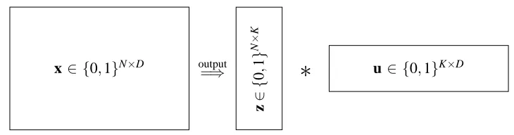
All sets in x have a vector representation in a D-dimensional Boolean space, where a 1 at dimen-sion d indicates the membership of item d in the respective set. D is the cardinality of the union of x1,x2, ...,xN. The matrix z∈ {0,1}N×K then indicates which subsets of u cover the sets in x: zik=1 indicates that uk covers xi. Using this notation, the set-covering problem is equivalent to

finding an exact Boolean decomposition of a binary matrix x with minimal K. An exact Boolean decomposition is x=z∗u, where the Boolean matrix product∗is defined such that

xid = K _

k=1

(zik∧ukd). (1)

Belohlavek and Vychodil (2010) show that the set cover problem is equivalent to Boolean factor analysis, where each factor corresponds to a row of u. Keprt and Snásel (2004) show that the factors together with the objects assigned to them can, in turn, be regarded as formal concepts as defined in the field of Formal Concept Analysis (FCA) by Ganter and Wille (1999). Stockmeyer (1975) shows that the set-cover problem is NP-hard and the corresponding decision problem is NP-complete. Since the set-cover problem is equivalent to the other problems, this also holds for Boolean factor analysis, finding the exact Boolean decomposition of a binary matrix, and FCA. Approximation heuristics exist and are presented below.

2.1.2 APPROXIMATEBOOLEANMATRIXDECOMPOSITION

An approximate decomposition of a matrix x is often more useful than an exact one. One can dis-tinguish two problems, which we refer to as the lossy compression problem (LCP) and the structure inference problem (SIP). For LCP, two different formulations exist. In the first formulation of Miet-tinen et al. (2006), the size of the matrix u is fixed and the reconstruction error is to be minimized.

Definition 2 (LCP1: Minimal Deviation for given K) For a given binary N×D matrix x and a given number K<min(N,D), find an N×K matrix z and a K×D matrix u such that the deviation

||x−z∗u||is minimal.

Alternatively, the deviation is given, as in Vaidya et al. (2007), and the minimal z and u must be found to approximate x.

Definition 3 (LCP2: Minimal K for Given Deviation) For a given binary N×D matrix x and a given deviationδ, find the smallest number K<min(N,D), a N×K matrix z, and a K×D matrix

x∈ {0,1}N×D

z

∈

{

0

,

1

}

N

×

K

u∈ {0,1}K×D

output

=⇒

∗

Figure 1: Dimensions of input data and output of the problems defined in Definitions 1–4.

The norm in both formulations of LCP is usually the Hamming distance. Both problems are NP-hard as shown by Vaidya et al. (2007).

In the structure inference problem (SIP), the matrix x is assumed to be generated from a structure part (z∗,u∗) and a random noise part. The goal is to find the decomposition (z∗,u∗) that recovers the structure and disregards the noise.

Definition 4 (SIP) Let the binary N×D matrix x be given. Assuming that x was generated from a hidden structure(z∗,u∗)and perturbed by noiseΘsuch that x∼p(x|Θ,z∗∗u∗), infer the underlying structure(z∗,u∗).

There is a substantial difference between SIP and the two lossy compression problems LCP1 and LCP2. Assuming that some of the entries are corrupted, neither the closest approximation of the original matrix nor the best compression is desirable. Instead, the goal is to infer a structure under-lying the data at hand rather than to decompose the matrix with the highest possible accuracy. Since the structure of the data is repeated across the samples, whereas its noise is irregular, better structure recovery will also provide better prediction of new samples or missing observations.

2.2 Approaches

Depending on the problem formulation, there are several ways how the factorization problems are approached. In this section we provide an overview over related methods.

2.2.1 COMBINATORIALAPPROACHES

2.2.2 MODEL-BASEDAPPROACHES

Solutions to the structure inference problem as presented in Wood et al. (2006), Šingliar and Hauskrecht (2006), Kabán and Bingham (2008), and Streich et al. (2009) are often based on probabilistic models. The likelihood that is most similar to the one we propose is the noisy-OR gate introduced in Pearl (1988). Our model allows random flips in both directions. The noisy-OR model, which is constrained to random bit flips from zeros to ones, is thus a special case of the noise model that we present in Section 3.2.4. A detailed comparison of the relationship between the noisy-OR model and our approach follows in Section 3.

There are two models that use a noisy-OR likelihood. Noisy-OR component analysis (NOCA), as in Šingliar and Hauskrecht (2006), is based on a variational inference algorithm by Jaakkola and Jordan (1999). This algorithm computes the global probabilities p(uj=1), but does not return a

complete decomposition. A non-parametric model based on the Indian-Buffet process (Griffiths and Ghahramani, 2011) and a noisy-OR likelihood is presented in Wood et al. (2006). We call this approach infinite noisy-OR (INO). Our method differs from INO with respect to the data likelihood and with respect to optimization. While our model yields an exact solution to an approximate model, replacing the binary assignments by probabilistic assignments, the inference procedure for INO aims at solving the exact model by sampling. INO is a latent feature model, as described by Ghahramani et al. (2007), with Boolean features. Latent feature models explain data by combinations of multiple features that are indicated as active (or inactive) in a binary matrix z. Being a member in multiple clusters (encoded in z) is technically equivalent to having multiple features activated.

Binary independent component analysis (BICA) of Kabán and Bingham (2008) is a factor model for binary data. The combination of the binary factors is modeled with linear weights and thus deviates from the goal of finding binary decompositions as we defined it above. However, the method can be adapted to solve binary decomposition problems and performs well under certain conditions as we will demonstrate in Section 5.2.

Two other model-based approaches for clustering binary data are also related to our model, al-though more distantly. Kemp et al. (2006) presented a biclustering method that infers concepts in a probabilistic fashion. Each object and each feature is assigned to a single bicluster. A Dirichlet process prior (Antoniak, 1974; Ferguson, 1973) and a Beta-Bernoulli likelihood model the assign-ments of the objects. Heller and Ghahramani (2007) presented a Bayesian non-parametric mixture model including multiple assignments of objects to binary or real-valued centroids. When an object belongs to multiple clusters, the product over the probability distributions of all individual mixtures is considered, which corresponds to the conjunction of the mixtures. This constitutes a probabilistic model of the Boolean AND, whereas in all the above methods mentioned, as well as in our model, the data generation process uses the OR operation to combine mixture components.

In this paper, we provide a detailed derivation and an in-depth analysis of the model that we proposed in Streich et al. (2009). We thereby extend the noise part of the model to several variants and unify them in a general form. Moreover, we provide an approach for the model-order selection problem.

2.3 Applications

associated data sets are clearly generated by multiple sources. Our model was motivated by this security-relevant problem. In the following, we will describe this problem and give representative examples of the main role mining methods that have been developed.

2.3.1 ROLEMINING ANDRBAC

The goal of role mining is to automatically decompose a binary user-permission assignment matrix

x into a role-based access control (RBAC) configuration consisting of a binary user-role assignment

matrix z and a binary role-permission assignment matrix u. RBAC, as defined in Ferraiolo et al. (2001), is a widely used technique for administrating access-control systems where users access sensitive resources. Instead of directly assigning permissions to users, users are assigned to one or more roles (represented by the matrix z) and obtain the permissions contained in these roles (represented by u).

The major advantages of RBAC over a direct user-permission assignment (encoded in the ma-trix x) are ease of maintenance and increased security. RBAC simplifies maintenance for two rea-sons. First, roles can be associated with business roles, i.e. tasks in an enterprise. This business perspective on the user is more intuitive for humans than directly assigning individual low-level permissions. Second, assigning users to just a few roles is easier than assigning them to hundreds of individual permissions. RBAC increases security over access-control on a user-permission level because it simplifies the implementation and the audit of security policies. Also, it is less likely that an administrator wrongly assigns a permission to a user. RBAC is currently the access control solution of choice for many mid-size and large-scale enterprises.

2.3.2 STRUCTURE ANDEXCEPTIONS INACCESSCONTROLMATRICES

The regularities of an access control matrix x, such as permissions that are assigned together to many users, constitute the structure of x. Exceptional user-permission assignments are not replicated over the users and thus do not contribute to the structure. There are three reasons for the existence of such exceptional assignments. First, exceptional assignments are often granted for ‘special’ tasks, for example if an employee temporarily substitutes for a colleague. Such exceptions may initially be well-motivated, but often the administrator forgets to remove them when the user no longer carries out the exceptional task. The second reason for exceptional assignments is simply administrative mistakes. Errors may happen when a new employee enters the company, or permissions might not be correctly updated when an employee changes position within the company. Finally, exceptional assignments can be intentionally granted to employees carrying out highly specialized tasks.

The role mining step should ideally migrate the regularities of the assignment matrix x to RBAC, while filtering out the remaining exceptional permission assignments. We model exceptional as-signments (all three cases) with a noise model described in Section 3.2. We are not aware of any way to distinguish these three cases when only user-permission assignments are given as an input. However, being able to separate exceptional assignments from the structure in the data substantially eases the manual search for errors.

2.3.3 PRIORART

(2008) apply an algorithm from formal concept analysis (see Ganter and Wille, 1999) to construct candidate roles (rows in u). The technique presented in Vaidya et al. (2007) uses an improved version of the database tiling algorithm from Han et al. (2000). In contrast to the method presented in Agrawal and Srikant (1994), their tiling algorithm avoids the construction of all concepts by using an oracle for the next best concept. A method based on a probabilistic model is proposed in Frank et al. (2008). The model is derived from the logical representation of a Boolean two-level hierarchy and is divided into several subcases. For one of the cases with only single assignments of objects, the bi-clustering method presented in Kemp et al. (2006) is used for inference.

3. Generative Model for Boolean Data from Multiple Sources

In this section we explain our model of the generation process of binary data, where data may be generated by multiple clusters. The observed data stems from an underlying structure that is perturbed by noise. We will first present our model for the structure and afterwards provide a unifying view on several noise processes presented in the literature.

We use a probabilistic model that describes the generative process. This has two advantages over discrete optimization approaches. First, considering a separate noise process for the irregularities of the data yields an interpretation for deviations between the input matrix x and its decomposi-tion(z,u). Second, the probabilistic representation of the sources u is a relaxation of the original computationally hard problem, as explained in the previous sections.

Let the observed data consist of N objects, each associated with D binary dimensions. More formally, we denote the data matrix by x, with x∈ {0,1}N×D_{. We denote the i}th _{row of the matrix} by xi∗, and the dthcolumn by x∗d. We use this notation for all matrices.

3.1 Structure Model

The systematic regularities of the observed data are captured by its structure. More specifically, the sources associated with the clusters generate the structure xS∈ {0,1}N×D_{. The association of}

data items to sources is encoded in the binary assignment matrix z∈ {0,1}N×K_{, with z}

ik=1 if and

only if the data item i belongs to the source k, and zik=0 otherwise. The sum of the assignment

variables for the data item i,∑kzik, can be larger than 1, which denotes that a data item i is assigned

to multiple clusters. This multiplicity gives rise to the name multi-assignment clustering (MAC). The sources are encoded as rows of u∈ {0,1}N×K_.

Let the set of the sources of an object be

L

possible assignment sets and

L

S

id is a Boolean

disjunction of the values at dimension d of all sources to which object i is assigned. The Boolean disjunction in the generation process of an xS_id results in a probability for x_idS =1, which is strictly non-decreasing in the number of associated sources|

L

L

dimension d, then x_idS =1. Conversely, xS_id =0 requires that all contributing sources have emitted a 0 in dimension d.

Let βkd be the probability that source k emits a 0 at dimension d: βkd := p(ukd =0). This

parameter matrixβ∈[0,1]K×D_{allows us to simplify notation and to write}

pS xSid =0|zi∗,β=

K

∏

k=1

βzik

kd and pS x S

The parameter matrixβencodes these probabilities for all sources and dimensions. Employing the notion of assignment sets, one can interpret the product

βL_id:= K

∏

k=1

βzik

kd (2)

as the source of the assignment set

L

single-assignment setting where L :=|L|independent sources are assumed and must be inferred.

Here, we only have K×D parametersβkd whereas in single-assignment clustering, the number of

source parameters would be L×D, which can be up to 2K×D. The expressionβL_id is rather a

‘proxy’-source, which we introduce just for notational convenience. The probability distribution of a xidgenerated from this structure model given the assignments

L

pS xSid|

L

= (1−βL_id)x

S

id(β_L

id)

1−xS_{id. (3)}

Note that we include the empty assignment set in the hypothesis class, i.e. a data item i need not belong to any class. The corresponding row xS_i∗contains only zeros and any element with the value 1 in the input matrix is explained by the noise process.

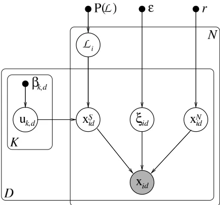
In the following sections, we describe various noise models that alter the output of the structure model. The structure part of the model together with a particular noise process is illustrated in Figure 2.

3.1.1 STRUCTURECOMPLEXITY ANDSINGLE-ASSIGNMENTCLUSTERING

In the general case, which is when no restrictions on the assignment sets are given, there are L= 2K possible assignment sets. If the number of clusters to which an object can be simultaneously assigned is bounded by M, this number reduces to L=∑M

m=0 Km

.

The particular case with M=1 provides a model variant that we call Single-Assignment Clus-tering (SAC). In order to endow SAC with the same model complexity as MAC, we provide it with L clusters. Each of the assignment sets is then identified with one of the clusters. The clusters are treated (and, in particular, updated) independently of each other by computing the cluster pa-rametersβL∗for each

L

L

com-puted according to Equation 2, the single-assignment clustering model yields the same probability for the data as the multi-assignment clustering model.

3.2 Noise Models and their Relationship

In this section, we first present the mixture noise model, which interprets the observed data as a mixture of independent emissions from the structure part and a noise source. Each bit in the matrix can thus be generated either by the structure model or by an independent global noise process. We then derive a more general formulation for this noise model. Starting there, we derive the flip model, where some randomly chosen bits of the signal matrix xS_{are flipped, either from 0 to 1 or from 1 to}

The different noise models have different parameters. We denote the noise parameters of a model α by Θα_N. The full set of parameters for structure and noise is then Θα := (β,Θα_N). As additional notation, we use the indicator function I_{p}for a predicate p, defined as

I{p}:=

1 if p is true 0 otherwise.

3.2.1 MIXTURENOISEMODEL

In the mixture noise model, each xid is generated either by the signal distribution or by a noise

process. The binary indicator variableξid indicates whether xid is a noisy bit (ξid =1) or a signal

bit (ξid=0). The observed xid is then generated by

xid= (1−ξid)xSid+ξidxNid ,

where the generative process for the signal bit xS

id is either described by the deterministic rule in

Equation 1 or by the probability distribution in Equation 3. The noise bit xN_id follows a Bernoulli distribution that is independent of object index i and dimension index d:

pN xidN |r

=rxNid(₁−_r)1−x N

id . ₍₄₎

Here, r is the parameter of the Bernoulli distribution indicating the probability of a 1. Combining the signal and noise distributions, the overall probability of an observed xid is

pmix_M (xid|

L

L

We assumeξidto be Bernoulli distributed with a parameterε:=p(ξid=1)called the noise fraction.

The joint probability of xidandξid given the assignment matrix z and all parameters is thus

pmix_M (xid,ξ|z,β,r,ε) =pM(xid|z,β,r,ξ)·εξid(1−ε)1−ξid.

Since different xid are conditionally independent given the assignments z and the parametersΘmix,

we have

pmix_M (x,ξ|z,β,r) =

∏

id

pmix_M (xid,ξ|z,β,r).

The noise indicators ξid cannot be observed. We therefore marginalize out all ξid to derive the

probability of x as

pmix_M (x|z,β,r,ε) =

∑

pmix_M (x,ξ|z,β,r,ε)

=

∏

id

(ε·pN(xid) + (1−ε)·pS(xid)).

The observed data x is thus a mixture between the emissions of the structure part (which has weight 1−ε) and the noise emissions (with weightε). Introducing the auxiliary variable

qmixL_id :=p_Mmix(xid=1|z,β,r,ε) =εr+ (1−ε) (1−βL_id)

to represent the probability that xid =1 under this model, we get a data-centric representation of the

probability of x as

pmix_M (x|z,β,r,ε) =

∏

id

(xidqmixL_id+ (1−xid) 1−qmixL_id

). (6)

Figure 2: The generative model of Boolean MAC with mixture noise.

L

object i, indicating which Boolean sources from u generated it. The bitξidselects whether

the noise-free bit xS_id or the noise bit xN_id is observed.

3.2.2 GENERALIZEDNOISEMODEL

In this section, we generalize the mixture noise model presented above. Doing so, we achieve a generalized formulation that covers, among others, the mentioned noisy-OR model.

The overall generation process has two steps:

1. The signal part of the data is generated according to the sources, as described in Section 3.1. It is defined by the probability pS xS_id|

L

(Equation 3).

2. A noise process acts on the signal xSand thus generates the observed data matrix x. This noise process is described by the probability pα(xid|x_idS,Θα_N), whereαidentifies the noise model and

Θα

N are the parameters of the noise modelα.

The overall probability of an observation xid given all parameters is thus

pα_M(xid|

L

∑

id

pS xSid|

L

·pα xid|xSid,ΘαN

.

3.2.3 MIXTURENOISEMODEL

The mixture noise model assumes that each xid is explained either by the structure model or by

an independent global noise process. Therefore, the joint probability of pmix xid|xS_id,ΘmixN

can be factored as

pmix xid|xSid,ΘmixN

=pmix_M xid|xSid,xNid,ξid

·pmix_N (xN_id|r),

with

pmix_M xid|xSid,xNid,ξid

=I_{xS

id=xid}

1−ξid

I_{xN

id=xid}

ξid

pS(xS_id|

L

N (xNid|r)are defined by Equation 3 and Equation 4 respectively. Summing out

the unobserved variables xS_id and xN_id yields

pmix_M (xid|

L

1

∑

xS

id=0

1

∑

xN

id=0

pmix_M xid,xSid,x N

id|

L

=pS(xid|

L

= (1−ξid)pS(xid|

L

Integrating out the noise indicator variablesξid leads to the same representation as in Equation 5.

3.2.4 FLIPNOISEMODEL

In contrast to the previous noise model, where the likelihood is a mixture of independent noise and signal distributions, the flip noise model assumes that the effect of the noise depends on the signal itself. The data is generated from the same signal distribution as in the mixture noise model. Individual bits are then randomly selected and flipped. Formally, the generative process for a bit xid

is described by

xid=xSid⊕ξid ,

where⊕denotes addition modulo 2. Again, the generative process for the structure bit xS_id is de-scribed by either Equation 1 or Equation 3. The value ofξid indicates whether the bit xSid is to be

flipped (ξid=1) or not (ξid=0). In a probabilistic formulation, we assume that the indicatorξid for

a bit-flip is distributed according toξid∼p(ξid|xS_id,ε0,ε1). Thus, the probability of a bit-flip, given the signal and the noise parameters(ε0,ε1), is

p(ξid|xSid,ε0,ε1) =

εxS id 1 ε

1−xS id 0

ξid

(1−ε1)x S

id(₁−ε

0)1−x S id

1−ξid

,

with the convention that 00=1. Given the flip indicatorξidand the signal bit xSid, the final

observa-tion is deterministic:

pflip_M (xid|ξid,xSid) =x I_{ξ

id6=xSid}

id (1−xid) I_{ξ

id=xSid} .

The joint probability distribution is then given by

pflip

xid|xSid,Θ

flip N = 1

∑

ξid=0

pflip_M (xid|ξid,xidS)·p(ξid|xSid,ε0,ε1).

3.2.5 RELATIONBETWEEN THENOISEPARAMETERS

Our unified formulation of the noise models allows us to compare the influence of the noise pro-cesses on the clean signal under different noise models. We derive the parameters of the flip noise model that is equivalent to a given mixture noise model based on the probabilities pmix(xid|xSid,ΘαN)

and pflip(xid|xS_id,ΘαN), for the cases(xid=1,xS_id=0)and(xid=0,xS_id=1):

The mixture noise model withΘmix_N = (ε,r)is equivalent to the flip noise model withΘflip_N = (ε·r,ε·(1−r)). Conversely, we have that the flip noise model withΘflip_N = (ε0,ε1)is equivalent to the mixture noise model withΘmix_N =ε0+ε1,_ε0ε₊0_ε1

Hence the two noise-processes are just different representations of the same process. We there-fore use only the mixture noise model in the remainder of this paper and omit the indicator αto differentiate between the different noise models.

3.2.6 OBJECT-WISE ANDDIMENSION-WISENOISEPROCESSES

In the following, we extend the noise model presented above. Given the equivalence of mix and flip noise, we restrict ourselves to the mixture noise model.

Dimension-wise Noise. Assume a separate noise process for every dimension d, which is

pa-rameterized by rd and has intensityεd. We then have

p(x|z,β,ε) =

∏

i,d

εdr_dxid(1−rd)1−xid+ (1−εd) (1−βL_id)xidβ1L−_idxid

.

Object-wise Noise. Now assume a separate noise process for every object i, which is

parame-terized byεiand ri. As before, we have

p(x|z,β,ε) =

∏

i,d

εirxiid(1−ri)1−xid+ (1−εi) (1−βL_id)xidβ1_L−xid

id

.

Note that these local noise models are very specific and could be used in the following appli-cation scenarios. In role mining, some permissions are more critical than others. Hence it appears reasonable to assume a lower error probability for the dimension representing, for example, root access to a central database server than for the dimension representing the permission to change the desktop background image. However we observed experimentally that the additional freedom in these models often leads to an over-parametrization and thus worse overall results. This problem could possibly be reduced by introducing further constraints on the parameters, such as a hierarchi-cal order.

4. Inference

We now describe an inference algorithm for our model. While the parameters are ultimately inferred according to the maximum likelihood principle, we use the optimization method of deterministic annealing presented in Buhmann and Kühnel (1993) and Rose (1998). In the following, we specify the deterministic annealing scheme used in the algorithm. In Section 4.2 we then give the character-istic magnitudes and the update conditions in a general form, independent of the noise model. The particular update equations for the mixture model are then derived in detail in Section 4.3.

4.1 Annealed Parameter Optimization

The likelihood of a data matrix x (Equation 6) is highly non-convex in the model parameters and a direct maximization of this function will likely be trapped in local optima. Deterministic annealing is an optimization method that parameterizes a smooth transition from the convex problem of maxi-mizing the entropy (i.e. a uniform distribution over all possible clustering solutions) to the problem of minimizing the empirical risk R. The goal of this heuristic is to reduce the risk of being trapped in a local optimum. Such methods are also known as continuation methods (see Allgower and Georg, 1980). In our case, R is the negative log likelihood. Formally, the Lagrange functional

is introduced, with Z being the partition function over all possible clustering solutions (see Equa-tion 10), and G denotes the Gibbs distribuEqua-tion (see EquaEqua-tion 9 and EquaEqua-tion 8). The Lagrange parameter T (called the computational temperature) controls the trade-off between entropy maxi-mization and minimaxi-mization of the empirical risk. Minimizing F at a given temperature T is equiva-lent to constraint minimization of the empirical risk R with a lower limit on the entropy H. In other words, H is a uniform prior on the likelihood of the clustering solutions. Its weight decreases as the computational temperature T is incrementally reduced.

At every temperature T , a gradient-based expectation-maximization (EM) step computes the parameters that minimize F. The E-step computes the risks RiL(Equation 7) of assigning data item

i to the assignment set

L

and

L

of the noise parameters. Then it uses these values to compute the optimal source parametersβ. The individual steps are described in Section 4.3.

We determine the initial temperature as described in Rose (1998) and use a constant cooling rate (T ←ϑ·T , with 0<ϑ<1) . The cooling is continued until the responsibilitiesγiLfor all data

items i peak sharply at single assignment sets

L

4.2 Characteristic Magnitudes and Update Conditions

Following our generative approach to clustering, we aim at finding the maximum likelihood solution for the parameters. Taking the logarithm of the likelihood simplifies the calculations as products be-come sums. Also, the likelihood function conveniently factors over the objects and features enabling us to investigate the risk of objects individually. We define the empirical risk of assigning an object i to the set of clusters

L

the sources contained in

L

RiL:=log p(xi·|

L

∑

log(xid(1−qLd) + (1−xid)qLd) . (7)

The responsibilityγiL of the assignment-set

L

γiL:=

exp(−RiL/T)

∑L′_∈

Lexp(−Ri

L′/T) . (8)

The matrixγdefines a probability distribution over the space of all clustering solutions. The ex-pected empirical riskEG[R]of the solutions under this probability distribution G is

EG[RiL] =

∑

i

∑

γiLRiL. (9)

Finally, the state sum Z and the free energy F are defined as follows.

Z :=

∏

i

∑

exp(−RiL/T) (10)

F :=−T log Z=−T

∑

i

log

∑

L

exp(−RiL/T)

!

any of the model parameters, i.e.θ∈β

µν,ε0,ε1,ε,r . Here, µ is some particular value of source index k andνis some particular value of dimension index d. Using this notation, the derivative of the free energy with respect toθis given by

∂F

∂θ =

∑

∑

γiL

∂RiL

∂θ =

∑

∑

γiL

∑

(1−2xid)∂qL_∂θd

xid(1−qLd) + (1−xid)qLd .

4.3 Update Conditions for the Mixture Noise Model

Derivatives for the mixture noise model (θ∈β

µν,ε,r ) are:

∂qmixL_d

∂βµν = (1−ε)βL\{µ},dI{ν=d}I{µ∈L},

∂qmixL_d

∂ε =1−r−βL_d,

∂qmixL_d

∂r =−ε.

This results in the following first-order conditions for the mixture noise model:

∂Fmix

∂βµν = (1−ε)L

∑

βL_\{µ},ν

(

∑i:xiν=1γ mix

iL

εr+ (1−ε) (1−βLν)

− ∑i:xiν=0γ mix

iL

1−εr−(1−ε) (1−βLν)

)

=0,

∂Fmix

∂ε =

∑

(

∑

L

(1−r−βL_d)∑_i:x

id=1γ

mix

iL

εr+ (1−ε) (1−βL_d) −

∑

L

(1−r−βL_d)∑_i:x

id=0γ

mix

iL

1−εr−(1−ε) (1−βL_d)

)

=0,

∂Fmix

∂r =ε

∑

(

∑

L

∑i:xid=0γ mix

iL

1−εr−(1−ε) (1−βL_d) −

∑

L

∑i:xid=1γ mix

iL

εr+ (1−ε) (1−βL_d)

)

=0.

There is no analytic expression for the solutions of the above equations, the parametersβµν,ε, and r are thus determined numerically. In particular, we use Newton’s method to determine the optimal values for the parameters. We observed that this method rapidly converges, usually needing at most 5 iterations.

The above equations contain the optimality conditions for the single-assignment clustering (SAC) model as a special case. As only assignment sets

L

model, we can globally substitute

L

element for multiplication, we getβL\{µ},ν=1.

In the noise-free case, the value for the noise fraction is ε=0. This results in a significant simplification of the update equations.

5. Experiments

In this section, we first introduce the measures that we employ to evaluate the quality of clustering solutions. Afterwards, we present results on both synthetic and real-world data.

5.1 Evaluation Criteria

quality criterion for the role mining problem. In the following, we introduce these two measures, parameter mismatch and generalization ability.

The following notation will prove useful. We denote by ˆz and ˆu the estimated decomposition of the matrix x. The reconstruction of the matrix based on this decomposition is denoted by ˆx, where ˆx :=ˆz∗ˆu. Furthermore, in experiments with synthetic data, the signal part of the matrix is known. As indicated in Section 3, it is denoted by xS.

5.1.1 PARAMETERMISMATCH

Experiments with synthetic data allow us to compare the values of the true model parameters with the inferred model parameters. We report below on the accuracies of both the estimated centroids ˆu and the noise parameters.

To evaluate the accuracy of the centroid estimates, we use the average Hamming distance be-tween the true and the estimated centroids. In order to account for the arbitrary numbering of clusters, we permute the centroid vectors uk∗ with a permutationπ(k)such that the estimated and the true centroids agree best. Namely,

a(ˆu):= 1

K·Dπmin∈PK

K

∑

k=1

u_k∗−uˆπ_(k)∗ ,

where PKdenotes the set of all permutations of K elements. Finding theπ∈PK that minimizes the

Hamming distance involves solving the assignment problem, which can be calculated in polynomial time using the Hungarian algorithm of Kuhn (2010). Whenever we know the true model parameters, we will assess methods based on parameter mismatch, always reporting this measure in percent.

5.1.2 GENERALIZATIONERROR

For real world data, the true model parameters are unknown and there might even exist a model mismatch between the learning model and the true underlying distribution that generated the input data set x(1). Still, one can measure how well the method infers this distribution by testing if the estimated distribution generalizes to a second data set x(2)that has been generated in the same way as x(1). To measure this generalization ability, we first randomly split the data set along the objects into a training set x(1)and a validation set x(2). Then we learn the factorization ˆz, ˆu based on the training set and transfer it to the validation set.

Note that the transfer of the learned solution to the validation set is not as straight-forward in such an unsupervised scenario as it is in classification. For transferring, we use the method proposed by Frank et al. (2011). For each object i in x(2), we compute its nearest neighborψNN(i)in x(1)

ac-cording to the Hamming distance. We then create a new matrix z′defined by z′_i∗=ˆz_ψNN(i)∗for all i. As a consequence, each validation object is assigned to the same set of sources as its nearest neigh-bor in the training set. The possible assignment sets as well as the source parameters are thereby restricted to those that have been trained without seeing the validation data. The generalization error is then

G(ˆz,ˆu,x(2),ψNN):=

1 N(2)_·D

x

(2)_−z′_∗ˆu ,

with z′=ˆz_ψNN(1)∗,ˆz_ψNN(2)∗, . . . ,ˆz_ψ

NN(N(2))∗

T

5 10 15 20 source 1

source 2 source 3

(a) Overlapping Sources (b) Orthogonal Sources

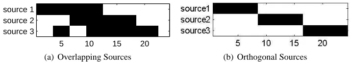
Figure 3: Overlapping sources (left) and orthogonal sources (right) used in the experiments with synthetic data. Black indicates a 1 and white a 0 for the corresponding matrix element. In both cases, the three sources have 24 dimensions.

where N(2)is the number of objects in the validation data set and∗is the Boolean matrix product as defined in Equation 1. This measure essentially computes the fraction of wrongly predicted bits in the new data set.

As some of the matrix entries in x(2)are interpreted as noise, it might be impossible to reach a generalization error of 0%. However, this affects all methods and all model variants. Moreover, we are ultimately interested in the total order of models with respect to this measure and not in their absolute scores. Since we assume that the noise associated with the features of different objects is independent, we deduce from a low generalization error that the algorithm can infer sources that explain—up to residual noise—the features of new objects from the same distribution. In contrast, a high generalization error implies that the inferred sources wrongly predict most of the matrix entries and thus indicates overfitting.

Note that the computation of generalization error differs from the approach taken in Streich et al. (2009). There, only ˆu is kept fixed, and ˆz is ignored when computing the generalization error. The assignment sets z′ of the new objects are recomputed by comparing all source combinations with a fractionκof the bits of these objects. The generalization error is the difference of the remaining (1−κ)bits to the assigned sources. In our experiments on model-order selection, this computation of generalization error led to overfitting. As z′ was computed independently from ˆz, fitting all possible role combinations to the validation data, it supports tuning one part of the solution to this data. With the nearest neighbor-based transfer of ˆz, which is computed without using the validation set, this is not possible. Overfitting is therefore detected more reliably than in Streich et al. (2009).

In order to estimate the quality of a solution, we use parameter mismatch in experiments with synthetic data and generalization error in experiments with real data.

5.2 Experiments on Synthetic Data

This section presents results from several experiments on synthetic data where we investigate the performance of different model variants and other methods. Our experiments have the following setting in common. First, we generate data by assigning objects to one or more Boolean vectors out of a set of predefined sources. Unless otherwise stated, we will use the generating sources as depicted in Figure 3. Combining the emissions of these sources via the OR operation generates the structure of the objects. Note that the sources can overlap, i.e. multiple sources emit a 1 at a particular dimension. In a second step, we perturb the data set by a noise process.

or-thogonal sources), the fraction of bits that are affected by the noise process, and the kind of noise process. Knowing the original sources used to generate the data set enables us to measure the accu-racy of the estimators, as described in Section 5.1. The goal of these experiments is to investigate the behavior of different methods under a wide range of conditions. The results will help us in interpreting the results on real-world data in the next section.

We repeat all experiments ten times, each time with different random noise. We report the median (and 65% percentiles) of the accuracy over these ten runs.

5.2.1 COMPARISON OFMACWITH OTHERCLUSTERING TECHNIQUES

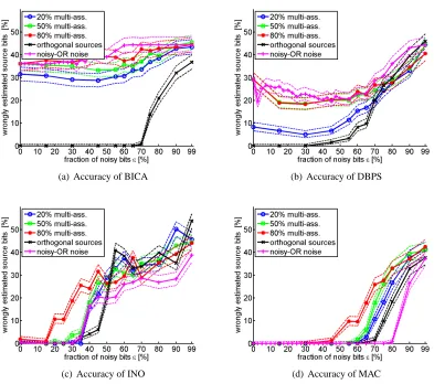
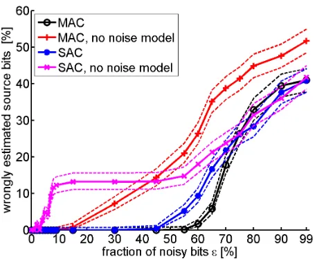
The main results of the comparison between MAC and other clustering techniques are shown in Figure 4. Each panel illustrates the results of one of the methods under five different experimental setups. We generate 50 data items from each single source as well as from each combination of two sources. Furthermore, 50 additional data items are generated without a source, i.e. they contain no structure. This experimental setting yields 350 data items in total. The overlapping sources are used as shown in Figure 3(a), and the structure is randomly perturbed by a mixture noise process. The probability of a noisy bit being 1 is kept fixed at r=0.5, while the fraction of noisy bits,ε, varies between 0% and 99%. The fraction of data from multiple sources is 50% for the experiments plotted with square markers. Experiments with only 20% (80%) of the data are labeled with circles (with stars). Furthermore, we label experiments with orthogonal sources (Figure 3(b)) with ’x’. Finally, we use ’+’ labels for results on data with a noisy-OR noise process, i.e. r=1.

5.2.2 BINARYINDEPENDENTCOMPONENTANALYSIS(BICA)

BICA has a poor parameter accuracy in all experiments with data from overlapping clusters. This behavior is caused by the assumption of orthogonal sources, which fails to hold for such data. BICA performs better on data that was modified by the symmetric mixture noise process than on data from a noisy-OR noise process. Since BICA does not have a noise model, the data containing noise from the noisy-OR noise process leads to extra 1s in the source estimators. This effect becomes important when the noise fraction rises above 50%. We observe that, overall, the error rate does not vary much for overlapping sources.

The effect of the source geometry is particularly noticeable. On data generated by orthogonal sources, i.e. when the assumption of BICA is fulfilled, the source parameters are perfectly recon-structed for noise levels up to 65%. Only for higher noise levels, does the accuracy break down. The assumption of orthogonal source centroids is essential for BICA’s performance as the poor results on data with orthogonal sources show. As more data items are generated by multiple, non-orthogonal sources, the influence of the mismatch between the assumption underlying BICA and the true data increases. This effect explains why the source parameter estimators for non-orthogonal centroids become less accurate when going from 20% of multi-assignments to 80%.

5.2.3 DISCRETEBASISPROBLEMSOLVER(DBPS)

(a) Accuracy of BICA (b) Accuracy of DBPS

(c) Accuracy of INO (d) Accuracy of MAC

Figure 4: Accuracy of source parameter estimation for five different types of data sets in terms of mismatch to the true sources. We use (circle, square, star) symmetric Bernoulli noise and overlapping sources with three different fractions of multi-assignment data, (x) or-thogonal sources and symmetric noise, and (+) overlapping sources and a noisy-or noise process. Solid lines indicate the median over 10 data sets with random noise and dashed lines show the 65% confidence intervals.

Note the effect of a small amount of noise on the accuracy of DBPS. The clear structure of the association matrix is perturbed, and the candidates might contain 0s in some dimensions. As a result, the roles selected in the second and subsequent steps are non-empty, making the solution more similar to the true sources. This results in the interesting effect where the accuracy increases when going from noise-free matrices to those with small amount of noise (for higher noise, it decreases again because of overfitting).

DBPS obtains accurate estimators in the setting where the data is generated by orthogonal data (labeled ’x’). Here, the candidate set does not contain sources that correspond to combinations of true sources, and the greedy optimization algorithm can only select a candidate source that corre-sponds to a true single source. DBPS thus performs best with respect to source parameter estimation when the generating sources are orthogonal. In contrast to BICA, which benefits from the explicit assumption of orthogonal sources, DBPS favors such sources because of the properties of its greedy optimizer.

5.2.4 INFINITE NOISY-OR (INO)

The infinite noisy-OR is a non-parametric Bayesian method. To obtain a single result, we ap-proximate the a posteriori distribution by sampling and then choose the parameters with highest probability. This procedure estimates the maximum a posterior solution. Furthermore, in contrast to BICA, DBPS, and all MAC variants, INO determines the number of sources by itself and might obtain a value different than the number of sources used to generate the data. If the number inferred by INO is smaller than the true number, we choose the closest true sources to compute the parameter mismatch. If INO estimates a larger set of sources than than the true one, the best-matching INO sources are used. This procedure systematically overestimates the accuracy of INO, whereas INO actually solves a harder task that includes model-order selection. A deviation between the estimated number of sources and the true number mainly occurs at the mid-noise level (approximately 30% to 70% noisy bits).

In all settings, except the case where 80% of the data items are generated by multiple sources, INO yields perfect source estimators up to noise levels of 30%. For higher noise levels, its accuracy rapidly drops. While the generative model underlying INO enables this method to correctly interpret data items generated by multiple sources, a high percentage (80%) of such data poses the hardest problem for INO.

For noise fractions above approximately 50%, the source parameter estimators are only slightly better than random in all settings. On such data, the main influence comes from the noise, while the contribution of different source combinations is no longer important.

5.2.5 MULTI-ASSIGNMENT CLUSTERING (MAC)

In comparison to the experiments with overlapping sources described in the previous paragraph, MAC profits from orthogonal centroids and yields superior parameter accuracy for noise levels above 50%. As for training data with little multi-assignment data, orthogonal centroids simplify the task of disentangling the contributions of the individual sources. When a reasonable first estimate of the source parameters can be derived from single-assignment data, a 1 in dimension d of a data item is explained either by the unique source which has a high probability of emitting a 1 in this dimension, or by noise—even if the data item is assigned to more than one source.

Interestingly, MAC’s accuracy peaks when the noise is generated by a noisy-OR noise process. The reason is that observing a 1 at a particular bit creates a much higher entropy of the parameter estimate than observing a 0: a 1 can be explained by all possible combinations of sources having a 1 at this position, whereas a 0 gives strong evidence that all sources of the object are 0. As a conse-quence, a wrong bit being 0 is more severe than a wrong 1. The wrong 0 forces the source estimates to a particular value whereas the wrong 1 distributes its ‘confusion’ evenly over the sources. As the noisy-OR creates only 1s, it is less harmful. This effect could, in principle, also help other methods if they managed to appropriately disentangle combined source parameters.

5.2.6 PERFORMANCE OFMAC VARIANTS

We carry out inference with the MAC model and the corresponding Single-Assignment Clustering (SAC) model, each with and without the mixture noise model. These model variants are explained in Section 3.1.1. The results illustrated in Figure 5 are obtained using data sets with 350 objects. The objects are sampled from the overlapping sources depicted in Figure 3(a). To evaluate the solutions of the SAC variants in a fair way, we compare the estimated sources against all combinations of the true sources.

5.2.7 INFLUENCE OFSIGNALMODEL ANDNOISEMODEL

As observed in Figure 5, the source parameter estimators are much more accurate when a noise model is employed. For a low fraction of noisy bits (<50%), the estimators with a noise model are perfect, but are already wrong for 10% noise when not using a noise model. When inference is carried out using a model that lacks the ability to explain individual bits by noise, the entire data set must be explained with the source estimates. Therefore, the solutions tend to overfit the data set. With a noise model, a distinction between the structure and the irregularities in the data is possible and allows one to obtain more accurate estimates for the model parameters.

Figure 5: Average Hamming distance between true and estimated source prototypes for MAC and SAC with and without noise models respectively.

We conducted the same experiments on data sets that are ten times larger and observed the same effects as the ones described above. The sharp decrease in accuracy is shifted to higher noise levels and appears in a smaller noise window when more data is available.

5.3 Experiments on Role Mining Data

To evaluate the performance of our algorithm on real data, we apply MAC to mining RBAC roles from access control configurations. We first specify the problem setting and then report on our experimental results.

5.3.1 SETTING ANDTASKDESCRIPTION

As explained in Section 2, role mining must find a suitable RBAC configuration based on a binary user-permission assignment matrix x. An RBAC configuration is the assignment of K roles to permissions and assignments of users to these roles. A user can have multiple roles, and the bit-vectors representing the roles can overlap. The inferred RBAC configuration is encoded by the Boolean assignment matrices(ˆz,ˆu).

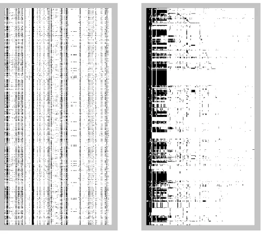
reg-Figure 6: A 2400×500 part of the data matrix used for model-order selection. Black dots indicate a 1 at the corresponding matrix element and white dots indicate a 0. The full data matrix has size 4900×1300. Rows and columns of the right matrix are reordered such that users with the same role set and permissions of the same role are adjacent to each other, if possible. Note that there does not exist a permutation that satisfies this condition for all users and permissions simultaneously.

ularities and irregularities. This is a problem for all role mining algorithms: The interpretation of the irregularities and any subsequent corrections must be performed by a domain expert. However, minimizing the number of suspicious bits and finding a decomposition that generalizes well is al-ready a highly significant advantage over manual role engineering. See Frank et al. (2010) for an extended discussion of this point.

In our experiments, we use a data set from our collaborator containing the user-permission assignment matrix of N=4900 users and D=1300 permissions. We will call this data set Corig in subsequent sections. A part of this data matrix is depicted in Figure 6. Additionally, we use the publicly available access control configurations from HP labs published by Ene et al. (2008).

(a) Generalization Error (b) run-time

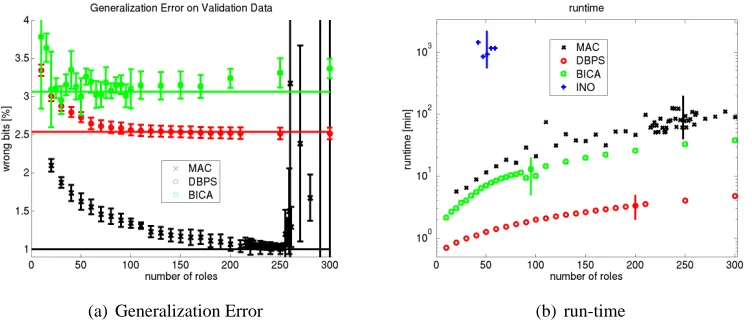
Figure 7: Left: Generalization error on the hold-out validation set in terms of wrongly predicted bits versus the number of roles. The other external parameters for BICA and DBPS are determined by exhaustive search. Right: Run-time versus number of roles on a 2400×

500 access-control matrix. The selected number of roles is highlighted by vertical lines.

5.3.2 MODEL-ORDERSELECTION

INO is a non-parametric model that can compute probabilities over the infinite space of all possible binary assignment matrices. It is therefore able to select the number of roles K during inference and needs no external input. For DBPS, BICA, and MAC, the number of roles must be externally selected and for DBPS and BICA, also rounding thresholds and approximation weights must be tuned. The number of roles K is the most critical parameter.

As a principle for guiding these model selection tasks, we employ the generalization error as defined in Section 5.1. Out of the total of 4900 users from Corig, we use five-fold cross-validation on a subset of 3000 users. In each step, we split them into 2400 users for training the model parameters and 600 users for validating them, such that each user occurs once in the validation set and four times in the training set. The number of permissions used in this experiment is 500. We increase the number of roles until the generalization error increases. For a given number of roles, we optimize the remaining parameters (of DBPS and BICA) on the training sets and validation sets. For continuous parameters, we quantize the parameter search-space into 50 equally spaced values spanning the entire range of possible parameter values.

Restricting the number of roles that can belong to a multiple assignment set risks having too few role combinations available to fit the data at hand. However, such circumstances cannot lead to underfitting when K is still to be computed in the cross-validation phase. In the worst case, an unavailable role combination would be substituted by an extra single role.

The performance of the three methods MAC, DBPS, and BICA as a function of the number of roles is depicted in Figure 7(a), left. The different models favor a substantially different number of roles on this data set (and also on other data sets, see Table 1). For MAC, there is a very clear indication of overfitting for K>248. For DBPS, the generalization error monotonically decreases for K<150. As K further increases, the error remains constant. In the cross-validation phase, the internal threshold parameter of DPBS is adapted to minimize the generalization error. This prevents excessive roles from being used as, with the optimal threshold, they are left empty. We select K=200 for DBPS, where more roles provide no improvement. INO selects 50 roles on average. BICA favors a considerably smaller number of roles, even though the signal is not as clear. We select K=95 for BICA, which is the value that minimizes the median generalization error on the validation sets.

5.3.3 RESULTS OFDIFFERENTMETHODS

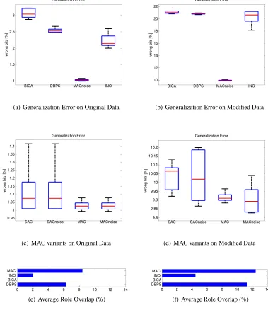
The results of the generalization experiments for the four methods MAC, DBPS, BICA, and INO are depicted in Figure 8. Overall, all methods have a very low generalization error on the original data set. The error spans from 1% to 3% of the predicted bits. This result indicates that, on a global scale, Corighas a rather clean structure. It should be stressed that most permissions in the input data set are only rarely assigned to users, whereas some are assigned to almost everyone, thereby making up most of the 1s in the matrix (see a part of the data set in Figure 6). Therefore, the most trivial role set where roles are assigned no permissions already yields a generalization error of 13.5%. Assigning everyone to a single role that contains all permissions that more than 50% percent of the users have, achieves 7.1%. One should keep this baseline in mind when interpreting the results.

INO, DBPS, and BICA span a range from 2.2% generalization error to approximately 3% with significant distance to each other. MAC achieves the lowest generalization error with slightly more than 1%. It appears that INO is misled by its noisy-OR noise model, which seems to be inappropriate in this case. MAC estimates the fraction of noisy bits by ˆε≈2.8% and the probability for a noisy bit to be 1 by ˆr≈20%. This estimate clearly differs from a noisy-OR noise process (which would have r=1). With more than 3% generalization error, BICA performs worst. As all other methods estimate a considerable centroid overlap, the assumption of orthogonal (non-overlapping) centroids made by BICA seems to be inappropriate here and might be responsible for the higher error.

In our experiments on the modified data set with more structure and a higher noise level, Fig-ure 8(b), all methods have significantly higher generalization errors, varying between approximately 10% to 21%. The trivial solution of providing each user all those permissions assigned to more than 50% of the users, leads to an error of 23.3%. Again, MAC with 10% generalization error yields significantly lower generalization error than all the other methods. INO, DBPS, and BICA perform almost equally well each with a median error of 20% to 21%. A generalization error of 10% is still very good as this data set contains at least 33% random bits, even though a random bit can take the correct value by chance.

(a) Generalization Error on Original Data (b) Generalization Error on Modified Data

(c) MAC variants on Original Data (d) MAC variants on Modified Data

(e) Average Role Overlap (%) (f) Average Role Overlap (%)

Figure 8: Generalization experiment on real data. Graphs (a)-(d) show the generalization error obtained with the inferred roles, and graphs (e)-(f) display the average overlap between roles.

5.3.4 RESULTS OFMAC MODELVARIANTS

To investigate the influence of the various model variants of MAC, we compare the performance reported above for MAC with i) the results obtained by the single-assignment clustering variant (SAC) of the model and ii) with the model variants without a noise part. The middle row of Figure 8 shows the generalization error of SAC and MAC, both with and without a noise model. On the original data set, Figure 8(c), all model variants perform almost equally well. The noise model seems to have little or no impact, whereas the multi-assignments slightly influence the generalization error. Taking MAC’s estimated fraction of noisy bits ˆε≈2.8% into account, we interpret this result by referring to the experiments with synthetic data. There the particular model variant has no influence on the parameter accuracy when the noise level is below 5% (see Figure 5.2.7). As we seem to operate with such low noise levels here, it is not surprising that the model variants do not exhibit a large difference on that data set. On the modified data with more complex structure and with a higher noise level than the original data (Figure 8(d)), the difference between multi-assignments and single-multi-assignments becomes more apparent. Both MAC and SAC benefit from a noise part in the model, but the multi-assignments have a higher influence.

5.3.5 RESULTS ONHP DATA

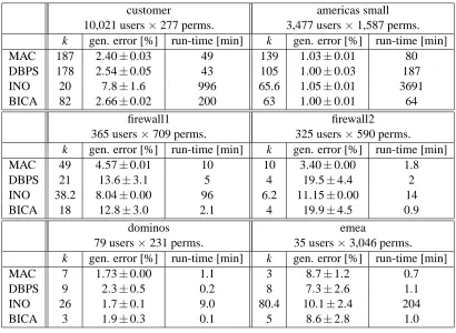
With all methods described above, we learn RBAC configurations on the publicly available data sets from HP labs (first presented by Ene et al., 2008). The data set ‘customer’ is the access control matrix of an HP customer. ‘americas small’ is the configuration of Cisco firewalls that provide users limited access to HP network resources. The data set ‘emea’ is created in a similar way and ‘firewall 1’ and ‘firewall 2’ are created by Ene et al. (2008) by analyzing Checkpoint firewalls. Finally, ‘domino’ is the access profiles of a Lotus Domino server.

We run the same analysis as on Corig. For the data sets ‘customer’, ‘americas small’, and ‘firewall 1’, we first make a trial run with many roles to identify the maximum cardinality of assignment sets M that MAC uses. We then restrict the hypothesis space of the model accordingly. For ‘customer’ and ‘firewall 1’, we use M=3, for ‘americas small’ we use M=2. For the smaller data sets, we simply offered MAC all possible role configurations, although the model does not populate all of them.

In the cross-validation phase we select the number of roles for each of the methods (except for INO), and the thresholds for BICA and DBPS in the previously described way. Afterwards we compute the generalization error on hold-out test data.