Exact Covariance Thresholding into Connected Components for
Large-Scale Graphical Lasso
Rahul Mazumder [email protected]
Trevor Hastie∗ [email protected]
Department of Statistics Stanford University Stanford, CA 94305
Editor: Francis Bach
Abstract
We consider the sparse inverse covariance regularization problem or graphical lasso with regular-ization parameterλ. Suppose the sample covariance graph formed by thresholding the entries of the sample covariance matrix atλis decomposed into connected components. We show that the
vertex-partition induced by the connected components of the thresholded sample covariance graph
(atλ) is exactly equal to that induced by the connected components of the estimated concentration graph, obtained by solving the graphical lasso problem for the sameλ. This characterizes a very interesting property of a path of graphical lasso solutions. Furthermore, this simple rule, when used as a wrapper around existing algorithms for the graphical lasso, leads to enormous performance gains. For a range of values ofλ, our proposal splits a large graphical lasso problem into smaller tractable problems, making it possible to solve an otherwise infeasible large-scale problem. We illustrate the graceful scalability of our proposal via synthetic and real-life microarray examples. Keywords: sparse inverse covariance selection, sparsity, graphical lasso, Gaussian graphical mod-els, graph connected components, concentration graph, large scale covariance estimation
1. Introduction
Consider a data matrix Xn×p comprising of n sample realizations from a p dimensional
Gaus-sian distribution with zero mean and positive definite covariance matrixΣp×p (unknown), that is,
xi i.i.d
∼ MVN(0,Σ),i=1, . . . ,n. The task is to estimate the unknown Σbased on the n samples. ℓ1
regularized Sparse Inverse Covariance Selection also known as graphical lasso (Friedman et al., 2007; Banerjee et al., 2008; Yuan and Lin, 2007) estimates the covariance matrixΣ, under the as-sumption that the inverse covariance matrix, that is,Σ−1is sparse. This is achieved by minimizing the regularized negative log-likelihood function:
minimize
Θ0 −log det(Θ) +tr(SΘ) +λ
∑
i,j|Θi j|, (1)where S is the sample covariance matrix. Problem (1) is a convex optimization problem in the
variableΘ(Boyd and Vandenberghe, 2004). LetΘb(λ) denote the solution to (1). We note that (1) can also be used in a more non-parametric fashion for any positive semi-definite input matrix S, not necessarily a sample covariance matrix of a MVN sample as described above.
A related criterion to (1) is one where the diagonals are not penalized—by substituting S← S+λIp×pin the “unpenalized” problem we get (1). In this paper we concentrate on problem (1).
Developing efficient large-scale algorithms for (1) is an active area of research across the fields of Convex Optimization, Machine Learning and Statistics. Many algorithms have been proposed for this task (Friedman et al., 2007; Banerjee et al., 2008; Lu, 2009, 2010; Scheinberg et al., 2010; Yuan, 2009, for example). However, it appears that certain special properties of the solution to (1) have been largely ignored. This paper is about one such (surprising) property—namely estab-lishing an equivalence between the vertex-partition induced by the connected components of the
non-zero pattern ofΘb(λ)and the thresholded sample covariance matrix S. This paper is not about a specific algorithm for the problem (1)—it focuses on the aforementioned observation that leads to a novel thresholding/screening procedure based on S. This provides interesting insight into the
path of solutions {Θb(λ)}λ≥0 obtained by solving (1), over a path of λ values. The behavior of
the connected-components obtained from the non-zero patterns of {Θb(λ)}λ≥0 can be completely
understood by simple screening rules on S. This can be done without even attempting to solve (1)— arguably a very challenging convex optimization problem. Furthermore, this thresholding rule can be used as a wrapper to enormously boost the performance of existing algorithms, as seen in our experiments. This strategy becomes extremely effective in solving large problems over a range of values ofλ—sufficiently restricted to ensure sparsity and the separation into connected components. Of course, for sufficiently small values ofλthere will be no separation into components, and hence no computational savings.
At this point we introduce some notation and terminology, which we will use throughout the paper.
1.1 Notations and Preliminaries
For a matrix Z, its(i,j)th entry is denoted by Z i j.
We also introduce some graph theory notations and definitions (Bollobas, 1998) sufficient for this exposition. A finite undirected graph
G
on p vertices is given by the ordered tupleG
= (V
,E
), whereV
is the set of nodes andE
the collection of (undirected) edges. The edge-set is equiv-alently represented via a (symmetric) 0-1 matrix1 (also known as the adjacency matrix) with p rows/columns. We use the convention that a node is not connected to itself, so the diagonals of the adjacency matrix are all zeros. Let|V
|and|E
|denote the number of nodes and edges respectively. We say two nodes u,v∈V
are connected if there is a path between them. A maximal connectedsubgraph2is a connected component of the graph
G
. Connectedness is an equivalence relation that decomposes a graphG
into its connected components{(V
ℓ,E
ℓ)}1≤ℓ≤K—withG
=∪Kℓ=1(V
ℓ,E
ℓ),where K denotes the number of connected components. This decomposition partitions the vertices
V
ofG
into {V
ℓ}1≤ℓ≤K. Note that the labeling of the components is unique upto permutationson {1, . . . ,K}. Throughout this paper we will often refer to this partition as the vertex-partition induced by the components of the graph
G
. If the size of a component is one, that is, |V
ℓ|= 1, we say that the node is isolated. Suppose a graphG
b defined on the set of verticesV
admits the following decomposition into connected components:G
b =∪Kbℓ=1(
V
bℓ,E
bℓ). We say thepartitions induced by the connected components of
G
andG
b are equal if Kb=K and there is apermutationπon{1, . . . ,K}such that
V
bπ(ℓ)=V
ℓfor allℓ∈ {1, . . . ,K}.The paper is organized as follows. Section 2 describes the covariance graph thresholding idea along with theoretical justification and related work, followed by complexity analysis of the algo-rithmic framework in Section 3. Numerical experiments appear in Section 4, concluding remarks in Section 5 and the proofs are gathered in the Appendix A.
2. Methodology: Exact Thresholding of the Covariance Graph
The sparsity pattern of the solution Θb(λ) to (1) gives rise to the symmetric edge matrix/skeleton
∈ {0,1}p×pdefined by:
E
(i jλ)=(
1 ifΘb(i jλ)6=0, i6=j;
0 otherwise. (2)
The above defines a symmetric graph
G
(λ)= (V
,E
(λ)), namely the estimated concentration graph(Cox and Wermuth, 1996; Lauritzen, 1996) defined on the nodes
V
={1, . . . ,p}with edgesE
(λ). Suppose the graphG
(λ)admits a decomposition intoκ(λ)connected components:G
(λ)=∪ℓκ=(λ1)G
ℓ(λ), (3)where
G
ℓ(λ)= (V
bℓ(λ),E
ℓ(λ))are the components of the graphG
(λ). Note thatκ(λ)∈ {1, . . . ,p}, withκ(λ) = p (largeλ) implying that all nodes are isolated and for small enough values of λ, there is only one component, that is,κ(λ) =1.
We now describe the simple screening/thresholding rule. Given λ, we perform a thresholding on the entries of the sample covariance matrix S and obtain a graph edge skeleton E(λ)∈ {0,1}p×p defined by:
E(i jλ)=
1 if|Si j|>λ, i6= j;
0 otherwise. (4)
The symmetric matrix E(λ)defines a symmetric graph on the nodes
V
={1, . . . ,p}given by G(λ)= (V
,E(λ)). We refer to this as the thresholded sample covariance graph. Similar to the decomposi-tion in (3), the graph G(λ)also admits a decomposition into connected components:G(λ)=∪ℓk=(λ1)G(ℓλ), (5)
where G(ℓλ)= (
V
ℓ(λ),E(ℓλ))are the components of the graph G(λ).Note that the components of
G
(λ)require knowledge ofΘb(λ)—the solution to (1). Constructionof G(λ)and its components require operating on S—an operation that can be performed completely independent of the optimization problem (1), which is arguably more expensive (See Section 3). The surprising message we describe in this paper is that the vertex-partition of the connected components of (5) is exactly equal to that of (3).
This observation has the following consequences:
2. The cost of computing the connected components of the thresholded sample covariance graph (5) is orders of magnitude smaller than the cost of fitting graphical models (1). Furthermore, the computations pertaining to the covariance graph can be done off-line and are amenable to parallel computation (See Section 3).
3. The optimization problem (1) completely separates into k(λ) separate optimization sub-problems of the form (1). The sub-problems have size equal to the number of nodes in each component pi :=|
V
i|,i=1, . . . ,k(λ). Hence for certain values ofλ, solvingprob-lem (1) becomes feasible although it may be impossible to operate on the p×p dimensional
(global) variableΘon a single machine.
4. Suppose that forλ0, there are k(λ0) components and the graphical model computations are distributed.3 Since the vertex-partitions induced via (3) and (5) are nested with increasingλ (see Theorem 2), it suffices to operate independently on these separate machines to obtain the
path of solutions{Θb(λ)}λfor allλ≥λ0.
5. Consider a distributed computing architecture, where every machine allows operating on a graphical lasso problem (1) of maximal size pmax. Then with relatively small effort we can
find the smallest value of λ=λpmax, such that there are no connected components of size larger than pmax. Problem (1) thus ‘splits up’ independently into manageable problems across
the different machines. When this structure is not exploited the global problem (1) remains intractable.
The following theorem establishes the main technical contribution of this paper—the equivalence of the vertex-partitions induced by the connected components of the thresholded sample covariance graph and the estimated concentration graph.
Theorem 1 For anyλ>0, the components of the estimated concentration graph
G
(λ), as defined in (2) and (3) induce exactly the same vertex-partition as that of the thresholded sample covari-ance graph G(λ), defined in (4) and (5). That isκ(λ) =k(λ)and there exists a permutation πon{1, . . . ,k(λ)}such that:
b
V
i(λ)=V
π((λi)), ∀i=1, . . . ,k(λ). (6)Proof The proof of the theorem appears in Appendix A.1.
Since the decomposition of a symmetric graph into its connected components depends upon the ordering/ labeling of the components, the permutationπappears in Theorem 1.
Remark 1 Note that the edge-structures within each block need not be preserved. Under a
match-ing reordermatch-ing of the labels of the components of
G
(λ)and G(λ):for every fixedℓsuch that
V
bℓ(λ)=V
ℓ(λ)the edge-setsE
(ℓλ)and E(ℓλ)are not necessarily equal.Theorem 1 leads to a special property of the path-of-solutions to (1), that is, the vertex-partition induced by the connected components of
G
(λ)are nested with increasingλ. This is the content ofthe following theorem.
Theorem 2 Consider two values of the regularization parameter such thatλ>λ′>0, with
corre-sponding concentration graphs
G
(λ) andG
(λ′)as in (2) and connected components (3). Then the vertex-partition induced by the components ofG
(λ)are nested within the partition induced by the components ofG
(λ′). Formally,κ(λ)≥κ(λ′)and the vertex-partition{
V
b(λ)ℓ }1≤ℓ≤κ(λ)forms a finer resolution of{
V
bℓ(λ′)}1≤ℓ≤κ(λ′).Proof The proof of this theorem appears in the Appendix A.2.
Remark 2 It is worth noting that Theorem 2 addresses the nesting of the edges across connected
components and not within a component. In general, the edge-set
E
(λ)of the estimated concentra-tion graph need not be nested as a funcconcentra-tion ofλ:forλ>λ′, in general,
E
(λ)6⊂E
(λ′).See Friedman et al. (2007, Figure 3), for numerical examples demonstrating the non-monotonicity of the edge-set acrossλ, as described in Remark 2.
2.1 Node-Thresholding
A simple consequence of Theorem 1 is that of node-thresholding. If λ≥maxj6=i|Si j|, then the ith node will be isolated from the other nodes, the off-diagonal entries of the ith row/column are all zero, that is, maxj6=i|Θb
(λ)
i j |=0. Furthermore, the ith diagonal entries of the estimated
covari-ance and precision matrices are given by (Sii+λ) and Sii1+λ, respectively. Hence, as soon as
λ≥maxi=1,...,p{maxj6=i|Si j|}, the estimated covariance and precision matrices obtained from (1)
are both diagonal.
2.2 Related Work
Witten et al. (2011) independently discovered block screening as described in this paper. At the time of our writing, an earlier version of their paper was available (Witten and Friedman, 2011); it proposed a scheme to detect isolated nodes for problem (1) via a simple screening of the entries of
S, but no block screening. Earlier, Banerjee et al. (2008, Theorem 4) made the same observation
about isolated nodes. The revised manuscript (Witten et al., 2011) that includes block screening became available shortly after our paper was submitted for publication.
Zhou et al. (2011) use a thresholding strategy followed by re-fitting for estimating Gaussian graphical models. Their approach is based on the node-wise lasso-regression procedure of Mein-shausen and B¨uhlmann (2006). A hard thresholding is performed on the ℓ1-penalized regression
3. Computational Complexity
The overall complexity of our proposal depends upon (a) the graph partition stage and (b) solving (sub)problems of the form (1). In addition to these, there is an unavoidable complexity associated with handling and/or forming S.
The cost of computing the connected components of the thresholded covariance graph is fairly negligible when compared to solving a similar sized graphical lasso problem (1)—see also our sim-ulation studies in Section 4. In case we observe samples xi∈ℜp,i=1, . . . ,n the cost for creating the
sample covariance matrix S is O(n·p2). Thresholding the sample covariance matrix costs O(p2). Obtaining the connected components of the thresholded covariance graph costs O(|E(λ)|+p) (Tar-jan, 1972). Since we are interested in a region where the thresholded covariance graph is sparse enough to be broken into smaller connected components—|E(λ)| ≪p2. Note that all computations pertaining to the construction of the connected components and the task of computing S can be computed off-line. Furthermore the computations are parallelizable. Gazit (1991, for example) describes parallel algorithms for computing connected components of a graph—they have a time complexity O(log(p))and require O((|E(λ)|+p)/log(p))processors with space O(p+|E(λ)|).
There are a wide variety of algorithms for the task of solving (1). While an exhaustive review of the computational complexities of the different algorithms is beyond the scope of this paper, we provide a brief summary for a few algorithms below.
Banerjee et al. (2008) proposed a smooth accelerated gradient based method (Nesterov, 2005) with complexity O(p4ε.5)to obtain anεaccurate solution—the per iteration cost being O(p3). They also proposed a block coordinate method which has a complexity of O(p4).
The complexity of the GLASSO algorithm (Friedman et al., 2007) which uses a row-by-row block coordinate method is roughly O(p3)for reasonably sparse-problems with p nodes. For denser problems the cost can be as large as O(p4).
The algorithm SMACSproposed in Lu (2010) has a per iteration complexity of O(p3) and an overall complexity of O(√p4ε)to obtain anε>0 accurate solution.
It appears that most existing algorithms for (1), have a complexity of at least O(p3) to O(p4) or possibly larger, depending upon the algorithm used and the desired accuracy of the solution— making computations for (1) almost impractical for values of p much larger than 2000.
It is quite clear that the role played by covariance thresholding is indeed crucial in this context. Assume that we use a solver of complexity O(pJ)with J∈ {3,4}, along with our screening proce-dure. Suppose for a givenλ, the thresholded sample covariance graph has k(λ) components—the total cost of solving these smaller problems is then∑ki=(λ1)O(|
V
i(λ)|J)≪O(pJ), with J∈ {3,4}. Thisdifference in practice can be enormous—see Section 4 for numerical examples. This is what makes large scale graphical lasso problems solvable!
4. Numerical Examples
4.1 Synthetic Examples
Experiments are performed with two publicly available algorithm implementations for the problem (1):
GLASSO: The algorithm of Friedman et al. (2007). We used the MATLAB wrapper available at
http://www-stat.stanford.edu/˜tibs/glasso/index.htmlto the Fortran code. The
specific criterion for convergence (lack of progress of the diagonal entries) was set to 10−5 and the maximal number of iterations was set to 1000.
SMACS: denotes the algorithm of Lu (2010). We used the MATLAB implementation
smooth_covsel available at http://people.math.sfu.ca/˜zhaosong/Codes/SMOOTH_
COVSEL/. The criterion for convergence (based on duality gap) was set to 10−5and the
max-imal number of iterations was set to 1000.
We will like to note that the convergence criteria of the two algorithmsGLASSOandSMACSare not the same. For obtaining the connected components of a symmetric adjacency matrix we used the MATLAB functiongraphconncomp. All of our computations are done in MATLAB 7.11.0 on a 3.3 GhZ Intel Xeon processor.
The simulation examples are created as follows. We generated a block diagonal matrix given by ˜S=blkdiag(˜S1, . . . ,˜SK), where each block ˜Sℓ=1pℓ×pℓ—a matrix of all ones and∑ℓpℓ=p. In the
examples we took all pℓs to be equal to p1(say). Noise of the formσ·UU′(U is a p×p matrix with
i.i.d. standard Gaussian entries) is added to ˜S such that 1.25 times the largest (in absolute value) off block-diagonal (as in the block structure of ˜S) entry ofσ·UU′equals the smallest absolute non-zero entry in ˜S, that is, one. The sample covariance matrix is S=˜S+σ·UU′.
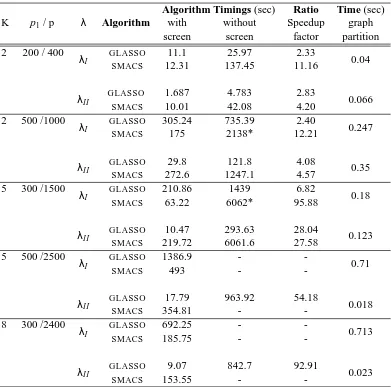
We consider a number of examples for varying K and p1values, as shown in Table 1. Sizes were
chosen such that it is at-least ‘conceivable’ to solve (1) on the full dimensional problem, without screening. In all the examples shown in Table 1, we setλI:= (λmax+λmin)/2, where for all values ofλin the interval[λmin,λmax]the thresh-holded version of the sample covariance matrix has exactly
K connected components. We also took a larger value ofλ, that is,λII:=λmax, which gave sparser estimates of the precision matrix but the number of connected components were the same.
The computations across different connected blocks could be distributed into as many machines. This would lead to almost a K fold improvement in timings, however in Table 1 we report the timings by operating serially across the blocks. The serial ‘loop’ across the different blocks are implemented in MATLAB.
K p1/ p λ Algorithm
Algorithm Timings (sec) Ratio Time (sec)
with without Speedup graph
screen screen factor partition
2 200 / 400 λI GLASSO 11.1 25.97 2.33
0.04
SMACS 12.31 137.45 11.16
λII GLASSO 1.687 4.783 2.83
0.066
SMACS 10.01 42.08 4.20
2 500 /1000 λI GLASSO 305.24 735.39 2.40
0.247
SMACS 175 2138* 12.21
λII GLASSO 29.8 121.8 4.08 0.35
SMACS 272.6 1247.1 4.57
5 300 /1500 λI GLASSO 210.86 1439 6.82
0.18
SMACS 63.22 6062* 95.88
λII GLASSO 10.47 293.63 28.04 0.123
SMACS 219.72 6061.6 27.58
5 500 /2500 λI GLASSO 1386.9 -
-0.71
SMACS 493 -
-λII GLASSO 17.79 963.92 54.18 0.018
SMACS 354.81 -
-8 300 /2400 λI GLASSO 692.25 -
-0.713
SMACS 185.75 -
-λII GLASSO 9.07 842.7 92.91
0.023
SMACS 153.55 -
-Table 1: -Table showing (a) the times in seconds with screening, (b) without screening, that is, on the whole matrix and (c) the ratio (b)/(a)—‘Speedup factor’ for algorithmsGLASSOand SMACS. Algorithms with screening are operated serially—the times reflect the total time summed across all blocks. The column ‘graph partition’ lists the time for computing the connected components of the thresholded sample covariance graph. SinceλII >λI, the former gives sparser models. ‘*’ denotes the algorithm did not converge within 1000 iterations. ‘-’ refers to cases where the respective algorithms failed to converge within 2 hours.
4.2 Micro-array Data Examples
see gracefully delivers solutions over a large range of the parameter λ. We study three different micro-array examples and observe that as one variesλfrom large to small values, the thresholded covariance graph splits into a number of non-trivial connected components of varying sizes. We continue till a small/moderate value of λwhen the maximal size of a connected component gets larger than a predefined machine-capacity or the ‘computational budget’ for a single graphical lasso problem. Note that in relevant micro-array applications, since p≫n (n, the number of samples is
at most a few hundred) heavy regularization is required to control the variance of the covariance estimates—so it does seem reasonable to restrict to solutions of (1) for large values ofλ.
Following are the data-sets we used for our experiments:
(A) This data-set appears in Alon et al. (1999) and has been analyzed by Rothman et al. (2008, for example). In this experiment, tissue samples were analyzed using an Affymetrix Oligonu-cleotide array. The data were processed, filtered and reduced to a subset of p=2000 gene expression values. The number of Colon Adenocarcinoma tissue samples is n=62.
(B) This is an early example of an expression array, obtained from the Patrick Brown Laboratory at Stanford University. There are n=385 patient samples of tissue from various regions of the body (some from tumors, some not), with gene-expression measurements for p=4718 genes.
(C) The third example is the by now famous NKI data set that produced the 70-gene prognostic signature for breast cancer (Van-De-Vijver et al., 2002). Here there are n=295 samples and
p=24481 genes.
Among the above, both (B) and (C) have few missing values—which we imputed by the respective global means of the observed expression values. For each of the three data-sets, we took S to be the corresponding sample correlation matrix. The exact thresholding methodolgy could have also been applied to the sample covariance matrix. Since it is a common practice to standardize the “genes”, we operate on the sample correlation matrix.
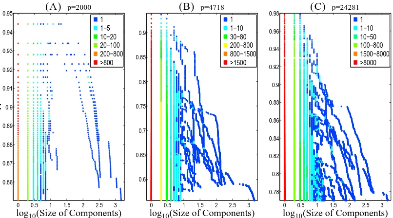
Figure 1 shows how the component sizes of the thresholded covariance graph change acrossλ. We describe the strategy we used to arrive at the figure. Note that the connected components change
only at the absolute values of the entries of S. From the sorted absolute values of the off-diagonal
0 0.5 1 1.5 2 2.5 3 0.86 0.87 0.88 0.89 0.9 0.91 0.92 0.93 0.94 0.95 1 1−5 10−20 20−100 200−800 >800 (A) p=2000 λ
log10(Size of Components)
0 0.5 1 1.5 2 2.5 3 0.6 0.65 0.7 0.75 0.8 0.85 0.9 1 1−10 30−80 200−800 800−1500 >1500 (B) p=4718
log10(Size of Components)
0 0.5 1 1.5 2 2.5 3 0.78 0.8 0.82 0.84 0.86 0.88 0.9 0.92 0.94 0.96 0.98 1 1−10 10−50 100−800 1500−8000 >8000 (C) p=24281
log10(Size of Components)
Figure 1: Figure showing the size distribution (in the log-scale) of connected components arising from the thresholded sample covariance graph for examples (A)-(C). For every value ofλ (vertical axis), the horizontal slice denotes the sizes of the different components appearing in the thresholded covariance graph. The colors represent the number of components in the graph having that specific size. For every figure, the range ofλvalues is chosen such that the maximal size of the connected components do not exceed 1500.
For examples (B) and (C) we found that the full problem sizes are beyond the scope of GLASSO andSMACS—the screening rule is apparently the only way to obtain solutions for a reasonable range ofλ-values as shown in Figure 1.
5. Conclusions
In this paper we present a novel property characterizing the family of solutions to the graphical lasso problem (1), as a function of the regularization parameterλ. The property is fairly surprising—the vertex partition induced by the connected components of the non-zero pattern of the estimated concentration matrix (atλ) and the thresholded sample covariance matrix S (atλ) are exactly equal. This property seems to have been unobserved in the literature. Our observation not only provides interesting insights into the properties of the graphical lasso solution-path but also opens the door to solving large-scale graphical lasso problems, which are otherwise intractable. This simple rule when used as a wrapper around existing algorithms leads to enormous performance boosts—on occasions by a factor of thousands!
Acknowledgments
Appendix A. Proofs
Here we provide proofs of Theorems 1 and 2.
A.1 Proof of Theorem 1
Proof SupposeΘb (we suppress the superscriptλ for notational convenience) solves problem (1), then standard KKT conditions of optimality (Boyd and Vandenberghe, 2004) give:
|Si j−cWi j| ≤λ ∀Θi jb =0; and (7)
c
Wi j=Si j+λ ∀Θi jb >0; Wci j=Si j−λ∀Θi jb <0; (8)
wherecW= (Θb)−1. The diagonal entries satisfycW
ii=Sii+λ, for i=1, . . . ,p.
Using (4) and (5), there exists an ordering of the vertices{1, . . . ,p}of the graph such that E(λ)is block-diagonal. For notational convenience, we will assume that the matrix is already in that order. Under this ordering of the vertices, the edge-matrix of the thresholded covariance graph is of the form:
E(λ)=
E(1λ) 0 ··· 0 0 E(2λ) 0 ···
..
. ... . .. ... 0 ··· 0 E(kλ(λ))
(9)
where the different components represent blocks of indices given by:
V
ℓ(λ), ℓ=1, . . . ,k(λ).We will construct a matrixcW having the same structure as (9) which is a solution to (1). Note
that ifcW is block diagonal then so is its inverse. LetcW and its inverseΘbbe given by:
c W= c
W1 0 ··· 0
0 cW2 0 ···
..
. ... . .. ... 0 ··· 0 cWk(λ)
, b Θ= b
Θ1 0 ··· 0
0 Θ2b 0 ···
..
. ... . .. ... 0 ··· 0 Θbk(λ)
Define the block diagonal matricescWℓor equivalentlyΘbℓvia the following sub-problems
b
Θℓ=arg min Θℓ
{−log det(Θℓ) +tr(SℓΘℓ) +λ
∑
i j
|(Θℓ)i j|} (10)
forℓ=1, . . . ,k(λ), where Sℓis a sub-block of S, with row/column indices from
V
ℓ(λ)×V
ℓ(λ). The same notation is used forΘℓ. Denote the inverses of the block-precision matrices by{Θbℓ}−1=cWℓ. We will show that the aboveΘb satisfies the KKT conditions—(7) and (8).Note that by construction of the thresholded sample covariance graph, if i∈
V
ℓ(λ)and j∈V
ℓ(′λ)withℓ6=ℓ′, then|Si j| ≤λ.Hence, for i ∈
V
ℓ(λ) and j∈V
ℓ(′λ) with ℓ6=ℓ′; the choice Θi jb =cWi j =0 satisfies the KKTconditions (7)
|Si j−cWi j| ≤λ
By construction (10) it is easy to see that for everyℓ, the matrixΘbℓsatisfies the KKT conditions (7) and (8) corresponding to the ℓth block of the p×p dimensional problem. Hence Θb solves
problem (1).
The above argument shows that the connected components obtained from the estimated preci-sion graph
G
(λ)leads to a partition of the vertices{V
b(λ)ℓ }1≤ℓ≤κ(λ)such that for everyℓ∈ {1, . . . ,k(λ)},
there is aℓ′∈ {1, . . . ,κ(λ)}such that
V
b(λ)ℓ′ ⊂
V
(λ)
ℓ . In particular k(λ)≤κ(λ).
Conversely, if Θb admits the decomposition as in the statement of the theorem, then it follows from (7) that:
for i∈
V
bℓ(λ) and j∈V
bℓ(′λ) with ℓ6=ℓ′; |Si j−cWi j| ≤λ. SincecWi j =0, we have|Si j| ≤λ. Thisproves that the connected components of G(λ)leads to a partition of the vertices, which is finer than the vertex-partition induced by the components of
G
(λ). In particular this implies that k(λ)≥κ(λ).Combining the above two we conclude k(λ) =κ(λ)and also the equality (6). The permutation
πin the theorem appears since the labeling of the connected components is not unique.
A.2 Proof of Theorem 2
Proof This proof is a direct consequence of Theorem 1, which establishes that the vertex-partitions
induced by the the connected components of the estimated precision graph and the thresholded sample covariance graph are equal.
Observe that, by construction, the connected components of the thresholded sample covariance graph, that is, G(λ)are nested within the connected components of G(λ′). In particular, the vertex-partition induced by the components of the thresholded sample covariance graph atλ, is contained inside the vertex-partition induced by the components of the thresholded sample covariance graph atλ′. Now, using Theorem 1 we conclude that the vertex-partition induced by the components of the estimated precision graph atλ, given by{
V
bℓ(λ)}1≤ℓ≤κ(λ)is contained inside the vertex-partitioninduced by the components of the estimated precision graph atλ′, given by{
V
bℓ(λ′)}1≤ℓ≤κ(λ′). The proof is thus complete.References
U. Alon, N. Barkai, D. A. Notterman, K. Gish, S. Ybarra, D. Mack, and A. J. Levine. Broad patterns of gene expression revealed by clustering analysis of tumor and normal colon tissues probed by oligonucleotide arrays. Proceedings of the National Academy of Sciences of the United States of
America, 96(12):6745–6750, June 1999. ISSN 0027-8424. doi: 10.1073/pnas.96.12.6745. URL
http://dx.doi.org/10.1073/pnas.96.12.6745.
O. Banerjee, L. El Ghaoui, and A. d’Aspremont. Model selection through sparse maximum likeli-hood estimation for multivariate gaussian or binary data. Journal of Machine Learning Research, 9:485–516, 2008.
B. Bollobas. Modern Graph Theory. Springer, New York, 1998.
D.R Cox and N. Wermuth. Multivariate Dependencies. Chapman and Hall, London, 1996.
J. Friedman, T. Hastie, and R. Tibshirani. Sparse inverse covariance estimation with the graphical lasso. Biostatistics, 9:432–441, 2007.
H. Gazit. An optimal randomized parallel algorithm for finding connected components in a graph.
SIAM Journal on Computing, 20(6):1046–1067, 1991.
S. Lauritzen. Graphical Models. Oxford University Press, 1996.
Z. Lu. Smooth optimization approach for sparse covariance selection. SIAM Journal on
Opti-mization, 19:1807–1827, February 2009. ISSN 1052-6234. doi: 10.1137/070695915. URL
http://portal.acm.org/citation.cfm?id=1654243.1654257.
Z. Lu. Adaptive first-order methods for general sparse inverse covariance selection. SIAM Journal
on Matrix Analysis and Applications, 31:2000–2016, May 2010. ISSN 0895-4798. doi: http:
//dx.doi.org/10.1137/080742531. URLhttp://dx.doi.org/10.1137/080742531.
N. Meinshausen and P. B¨uhlmann. High-dimensional graphs and variable selection with the lasso.
Annals of Statistics, 34:1436–1462, 2006.
Y. Nesterov. Smooth minimization of non-smooth functions. Mathematical Programming, Series
A, 103:127–152, 2005.
A.J. Rothman, P.J. Bickel, E. Levina, and J. Zhu. Sparse permutation invariant covariance estima-tion. Electronic Journal of Statistics, 2:494–515, 2008.
K. Scheinberg, S. Ma, and D. Goldfarb. Sparse inverse covariance selection via alternating lin-earization methods. In Neural Information Processing Systems, pages 2101–2109, 2010.
R. E. Tarjan. Depth-first search and linear graph algorithms. SIAM Journal on Computing, 1(2): 146160, 1972.
M. J. Van-De-Vijver, Y. D. He, L. J. van’t Veer, H. Dai, A. A. Hart, D. W. Voskuil, G. J. Schreiber, J. L. Peterse, C. Roberts, M. J. Marton, M. Parrish, D. Atsma, A. Witteveen, A. Glas, L. Delahaye, T. van der Velde, H. Bartelink, S. Rodenhuis, E. T. Rutgers, S. H. Friend, and R. Bernards. A gene-expression signature as a predictor of survival in breast cancer. The New England Journal
of Medicine, 347:1999–2009, Dec 2002.
D. Witten and J. Friedman. A fast screening rule for the graphical lasso. accepted for publication
in Journal of Computational and Graphical Statistics, 2011. Report dated 5-12-2011.
D. Witten, J. Friedman, and N. Simon. New insights and faster computations for the graphical lasso.
Journal of Computational and Graphical Statistics, 20(4):892–900, 2011. (Reference draft dated
9/8/2011).
M. Yuan and Y. Lin. Model selection and estimation in the gaussian graphical model. Biometrika, 94(1):19–35, 2007.
X. Yuan. Alternating direction methods for sparse covariance selection. Methods, (August):1–12,