Please cite this article in press asBabalola B.T and Yahya W. B. Effects of Collinearity on Cox Proportional Hazard Model with Time Dependent Coefficients: A Simulation Study. J Biostat Epidemiol. 2019; 5(2): 172-182
J Biostat Epidemiol. 2019;5(1): 172-182
Original Article
Effects of Collinearity on Cox Proportional Hazard Model with Time Dependent
Coefficients: A Simulation Study
B. T. Babalola1* and W. B. Yahya2
1Department of Statistics, Ekiti State University, Ado- Ekiti, Nigeria. 2Department of Statistics,University of Ilorin, Ilorin, Nigeria.
ARTICLE INFO ABSTRACT
Received 12.02.2019 Revised 15.03.2019 Accepted 14.04.2019 Published 01.05.2019
Key words: Baseline hazard; Time-dependent coefficient; Collinearity; Schoenfeld residuals
Background: The Cox proportional hazard model has gained ground in Biostatistics and other related fields. It has been extended to capture different scenarios, part of which are violation of the proportionality of the hazards, presence of time dependent covariates and also time dependent co-efficients. This paper focuses on the behaviour of the Cox Model in relation to time coefficients in the presence of different levels of collinearity.
Objectives: The objectives of this study are to examine the effects of collinearity on the estimates of time dependent co-effiecients in Cox proportional hazard model and to compare the estimates of the model for the logarithm and the square functions of time.
Materials and methods: The Algorithm based on a binomial model was extended in order to incorporate the different correlation structures required for the study. The scaled Schoenfeld residuals plots revealed the behaviour of the estimated betas at different degrees of collinearity. Results and conclusions are based of outcome of simulation study performed only.
Results: The estimated betas were compared to the true betas at the different level of collinearity in graphical pattern.
Conclusion: The study shows that collinearity is a huge factor that influences the correctness of the estimates of the regressors within the framework of Cox model.
Introduction
Cox regression model which takes into account the effect of censored observations is one the most applicative and used models in survival analysis to evaluate the effects of covariates. The choice of time function in extended Cox regression model was considered for investigation.[1] The extension of the Cox proportional hazard method for estimating survival time has been an attractive area of research in recent years.[2] An extension of the classical Cox proportional hazard model gave birth to the introduction of the time dependency nature of some data. Considering the predictors
* Corresponding Author: teniola.babalola@eksu.edu.ng
173 wishes to examine the link between area of
residence and cancer, this would be complicated by the fact that study subjects move from one area to another. The area of residency could then be introduced in the statistical model as a time-varying covariate. Some time-dependent variables in survival analyses models are income, marital status, location, or treatment. A large
family of models which focuses directly on the hazard function was introduced. [4] The simplest member of the family is the proportional hazard model, where the hazard at time t for an individual with covariates xi(not including a constant) is assumed to be
' 0( )exp )
|
( i i
i t x t x (1) In this model
0(
t
)
is a baseline hazardfunction that describes the risk for individuals with xi=0,who serves as a reference cell or pivot, and
'
exp xi is the relative risk, a proportionate
increase or decrease in risk, associated with the set of characteristics xi. Note that the increase or reduction in the risk is the same at all duration t. When time-dependent covariates are considered, the model becomes:
2 1 1 10
(
)
exp
(
)
)
)
(
|
(
p j j j i p i ii
t
X
t
t
X
X
t
(2) Even though the values of the variable X j (t)
may change over time, the hazard model provides only one coefficient for each time-dependent variable in the model. Thus, at time t, there is only one value of the variable X j (t) that has an effect on the hazard, that value being measured at time
t.
i and
jare the coefficients of time independent and the time dependent variables respectively.In a scenario with only time-dependent covariates, we have
1 10
(
)
exp
(
)
)
)
(
|
(
p j j ji
t
X
t
t
X
t
(3) Mathematically, it is possible to move from a
time dependent covariate while the relationship
with time is a function of time (say g(t)) to a time dependent coefficient as follows:
1 10
(
)
exp
(
)
)
)
(
|
(
p j j ji
t
X
t
t
X
t
1 10( )exp ( ( )) ) ) ( | ( p j j j j
i t X t
t
X g t
1 10
(
)
exp
(
(
))
)
)
(
|
(
p j j j ji
t
X
t
t
g
t
X
1 1 0(
)
exp
(
)
)
)
(
|
(
p j j ji
t
X
t
t
t
X
(4) The last equation is an Extended Cox model
for time dependent coefficients. The application of the Cox model requires the validation of the proportional hazard model assumption. There are
174 Several methods have been proposed for
checking the predictor for time dependency. Many graphical approaches have been proposed to check for proportionality. Although, the judgment if rather subjective and can be used as a first guide. Some of which are: the Kaplan-Meier curves for parallelism, the Schoenfeld Residual plot to mention a few. Smoothing spline and Fractional polynomial provide a means of obtaining the functional estimate of time variation. Isotonic regression as a method of solving the function of time was introduced. Another assumption is the issue of non-informative censoring. To satisfy this assumption, the design of the underlying study must ensure that the mechanisms giving rise to censoring of individual subjects are not related to the probability of an event occurring. For example, in clinical studies, care must be taken that continuation of follow-up not depend on a participants medical condition. [5]
Collinearity is a term used to describe a situation where by two variables are correlated.[6] In Regression analysis, Collinearity can increase estimates of parameter variance; yield models in which no variable is statistically significant even though
2
i
R
is large; produce parameter estimates of the “incorrect sign” and of implausible magnitude; create situations in which small changes in the data produce wide swings in parameter estimates; and, in truly extreme cases, prevent the numerical solution of a model. These problems can be severe and sometimes crippling. Multicollinearity has an equivalent effect and it occurs when more than two variables are correlated. [7],[8],[9] and [10]
The paper presents the effects of collinearity on the estimates time-dependent coefficients of the Cox proportional hazard model using the log and square of time functions. The true values and the estimates by Cox model were compared using graphs for the two different functions of time. A simulation study was employed for the research.
Review of Literature
Some researches worked on Cox regression analysis in presence of collinearity. In their paper, they considered the analysis of time to event data in the presence of collinearity between covariates. They bent toward the ridge estimator because in linear and logistic regression, used as an alternative to the maximum likelihood estimator in the presence of multicollinearity. Based on the fact that the ridge regression estimator has some desired properties like having a small total mean square error, they generalized this approach for addressing collinearity to the Cox proportional hazards model. Simulation studies were conducted to evaluate the performance of the ridge regression estimator. They did not consider time dependent coefficients.[11]
Murphy and Sen(1991) worked on the estimation of time-varying coefficient in a Cox-type parameterization of the stochastic intensity of point process. They made use of sieve estimation procedure(Grenander, 1981) to estimate the coefficient. A rate of convergence in probability for the sieve estimation was given and a functional central limit theorem for the integrated sieve estimator was proved.[3]
Zhangsheng and Xihong (2010) proposed a working independent profile likelihood method for the semi-parametric time-varying coefficient model with correlation. Kernel likelihood was used to estimate time-varying coefficients. Profile likelihood for the parametric coefficients was formed by plugging in the nonparametric estimator. For independent data, the estimator was asymptotically normal and achieves the asymptotic semi-parametric efficiency bound. They evaluated the performance of proposed nonparametric kernel estimator and the profile estimator, and apply the method to the western Kenya parasitemia data.[12]
175 well-known functions of standard Brownian
motion, leading to the construction of formal goodness-of-fit tests. Some numerical studies were included to illustrate the performance of the tests for moderate sample sizes.[13]
Sylvestre and Abrahamowicz (2007), made a comparison of algorithm for generating event times conditional on time dependent covariates. They examined the Permalgorithm (PAs) and the Binomial algorithm they modified the PAs to incorporate the rejection sampler. They performed a simulation study to assess the accuracy, stability and the speed of the algorithms. It was concluded that both algorithms data sets that, once analyzed, provided virtually unbiased estimates with comparable variances.[14]
Zhu et al (2017), were interested in reporting and methodological quality of survival analysis in articles published in Chinese oncology journals. In their work they mentioned that collinearity often exists in independent covariates in cox models.[1]
Vatcheva et al (2018), worked on multicollinearity in regression analyses conducted in epidemiologic studies. They demonstrated the adverse effects of multicollinearity in the regression analysis and encourage researchers to consider the diagnostic for multicollinearity as one of the steps in regression analysis.[15]
Some other relevant works that are informative and are related to the research which may be beneficial to reader can be seen in the following: [16],[17] and [18].
An Algorithm based on binomial model (Binomial Algorithm)
This is an algorithm based on the binomial model. The binomial algorithm requires that the continuous follow-up time is partitioned into a finite number of m time intervals, which is assumed were of equal length. The algorithm involves three steps, performed iteratively from time t=1 to either the end of follow-up (t=m) or the time the individual is assigned the event or censored, separately for each individual i =1,...,n still at risk:
Compute the individual conditional probability of event Pi,t, based on a binomial
model with parameters
j, j=1,2,…,w. corresponding to those of equation (1).
wj
i j j t
i
X
t
P
it
(
)
(
)
log
,
0
,Generate Ui,tfrom
U
[
0
,
1
]
If Ui,t Pi,t , assign an event to subject i at time t, Ti=t , and stop the follow-up for this
subject. Otherwise, increase t by 1 unit and return to step 1.
The pre-specified value of logit(
0)represents the baseline risk, i.e. the probability of an event for an individual with all covariate values set at 0. A baseline risk that is constant over time implies event times that are exponentially distributed. The higher the baseline risk, the bigger P, the probability of event at a given time, is, and the more likely that events will be generated early in the follow-up. However, it is difficult to control the exact form of the resulting distribution of the generated event times.
Simulation Scheme
176 and 2 for
X
1 andX
2 respectively using R code.The R-software was used for all simulation and analysis.
Two basic functions of time were considered that is the logarithm of time and the square of
time. For the time dependent beta (td.beta) for the logarithm of time is given below. The first variable is considered as a reference variable however it is still has a time dependent coefficient. Time-dependent regression coefficients were simulated.
td.beta1 = 0.01t+0.001t2
td.beta2= 0.1log(t) (*) For the other function, we have
td.beta1 = 0.01t+0.001t2
td.beta2= 0.001 t2 (**) Equations (*) and (**) were chosen in order to have a reduced scale of time for the two functions of time.
Results
The results of the study are presented in this section. The reference covariate is first discussed. Subsequently, the logarithm of time was discussed and the square of time. The figures below show the effect collinearity has on the estimates of a time dependent coefficient.
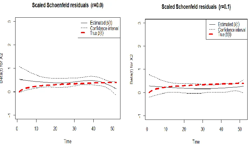
The scaled schoenfeld plots of the reference covariate(X1) for the two different combinations of functions of time in the absence of collinearity. Fig. 1
The scaled Schoenfeld plots of the reference covariate(X1) for the two different combinations
of functions of time in the presence of
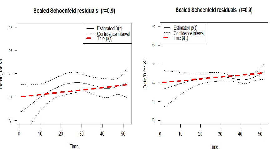
177 Fig. 2
This shows the scaled schoenfeld residuals of the two reference covariates at no collinearity and
at high level of collinearity.( log of time was considered here).
Fig.3
This shows the scaled Schoenfeld residuals of the two reference covariates at no collinearity and
178 Fig. 4
For the log of time, we have the following: This shows the scaled schoenfeld residuals of the two reference covariates at no collinearity and at high level of collinearity (log of time was considered here).
These are the plots of the scaled Schoenfeld residuals of some other levels of collinearity of the covariate with time dependent coefficient carrying a log function of time.
179 Considering the square of time, we have the
181
Discussion
The effects of collinearity in the estimation of time dependent coefficients cannot be hidden. For the two cases considered, the effect of collinearity appeared to be the same as it increases the spread of the confidence interval as the correlation between the variables increases. This is very apparent in figures 1 and 2. In figure 1(a), which shows the scaled Schoenfeld residuals in the absence of collinearity in the reference covariate, the true beta (
t
) is close to the estimated betas .The estimated betas all fall within the confidence interval as well. Whereas, as for figure 1(b), it is not until towards the end that the true value was not captured by the confidence interval in its entirety. In figure 2 (at a very high level of collinearity, r=0.9) , the estimated betas do not have the same pattern with the true betas and the spread of the confidence interval is extremely high . This shows that the effect of collinearity on the estimate is high as such there is a reduction in the efficiency of the Cox model in the presence of a high level of collinearity. This is obvious in both figures 2 (a) and 2(b).A close look at figure 3 clearly reveals the difference in the estimated betas when the collinearity level is high and when it is absent and when the log transformation of time is involved. At no collinearity, the estimated betas and the true betas are close unlike the other part when correlation is 0.9. Like the reference variable, the spread of the confidence interval increases as correlation increases. Even when the time transformation considered was square of time, the results obtained still follows the same pattern as the others have been. Closeness of the estimated betas to the true beta reduces as correlation increases and the band of the confidence interval becomes wider.
For the log of time as displayed in figure 7, the erratic behavior of the estimated betas became more obvious as the level of collinearity increases. For the square of time scenario, underestimation of the parameters is apparent and the pattern of the estimated betas seems to be
more uniform when compared to that of logarithm of time but the higher the level of collinearity, the farther the estimates of betas from the true betas.
Conclusion
The study reveals the effects of collinearity on the estimates of time dependent coefficient. It indicates that deflection from the true values of betas increases as the level of correlation between the variables increase regardless of the function of time considered. These are indicated in the plots. This can be generalized to cases when we have more than two variables and also when we consider other different functions of time. The scaled Schoenfeld residuals plots were used to illustrate the violation of the proportionality assumption of the Cox model. We have been able to show through this study that collinearity is a huge factor that influences the correctness of the estimates of the regressors within the framework of Cox model.
Reference
1. Zhu X, Zhou X, Zhang Y, Sun X, Liu H, Zhang Y. Reporting and methodological quality of survival analysis in articles published in Chinese oncology journals. Medicine[Internet]. 2017 Dec;
96(50):1-7. Available from:
https://www.ncbi.nlm.nih.gov/pubmed/2939034 0
2. Husain H, Thamrin SA, Tahir S, Mukhlisin A, Apriani MM (2018) The application of extended Cox proportional hazard method for estimating survival time of breast cancer. J of Phys [Internet]. 2018; the 2nd International Conference on Science. Conference Series 979
012087. Available from:
https://iopscience.iop.org/article/10.1088/1742-6596/979/1/012087
182
39(1):153-180. Available from:
https://www.sciencedirect.com/science/article/pi i/030441499190039F
4. Cox DR. Regression models and life-tables (with discussion). J of the Royal Stat Soc, Series B: Methodological [Internet]. 1972; 34(1) 187–
220. Available from:
https://www.jstor.org/stable/
5. Salanti G, Ulm K. A non-parametric change point model for stratifying continuous variables under order restrictions and binary outcome. Stat methods in med research[Internet]. (2003); 12(1):351-367. Available from: https://rmgsc.cr.usgs.gov/outgoing/threshold_art icles/Salanti_Ulm2003.pdf
6. Yahya WB, Olaifa JB. A note on Ridge Regression Modeling Techniques. Elect J of App Stat Ana,[Internet]. (2014); 7(2):343-361.
Available from:
http://siba-ese.unisalento.it/index.php/ejasa/article/view/12 502
7. Belsley DA. Assessing the presence of harmful collinearity and other forms of weak data through a test for signal-to-noise. J of Econ [Internet].1980; 20(1): 211-253. Available from:
https://link.springer.com/article/10.1007%2FBF 00426854
8. Belsley DA, Kuh E, Welsch RE. Regression Diagnostics. Identifying Influential Data and Sources of Collinearity. New York: John Wiley & Sons.
9. Greene WH. (1993): Econometric Analysis. Englewood Cliffs, NJ: Prentice-Hall.
10. Garba MK, Oyejola BA and Yahya WB. Investigation of Certain Estimators for Modeling Panel Data under Violations of Some Basic Assumptions. Math Theory and Mod [Internet]. 2013 (3)10: 47-53. Available from: https://issuu.com/unilorinbulletin/docs/270114 11. Xue X, Kim MY, Shore RE Cox regression analysis in presence of collinearity: an application to assessment of health risks associated with occupational radiation exposure. Pubmed [Internet]. 2007 Sep; 13(3): 333-350.
Available from:
https://www.cdc.gov/niosh/nioshtic-2/20040338.html
12. Zhangsheng Y, Xihong L(2010). Semi-parametric regression with time-dependent coefficients for failure time data analysis. Statistica Sinica [Internet]. 2010; 20(1); 853-869.
Available from:
https://www.ncbi.nlm.nih.gov/pmc/articles/PMC 2877509/
13. Marzec L, Marzec P. Generalized martingale-residual processes for goodness-of-fit inference in Cox's type regression models. The ann of stat [Internet]. 1997; 25(2): 683-714. Available from: https://projecteuclid.org/euclid.aos/1031833669 14. Sylvestre MP, Abrahamowicz M. Comparison of algorithms to generate event times conditional on time-dependent covariates. Statist. Med. [Internet]. 2008; 27: 2618–2634. Available from:
https://www.ncbi.nlm.nih.gov/pmc/articles/PMC 3546387/
15. Vatcheva KP, Lee M, McCormick JB, Rahbar MH. Multicollinearity in Regression Analyses Conducted in Epidemiologic Studies. Epidemiol [Internet]. 2016 Apr; 6(2):227-232.Available from:
https://www.ncbi.nlm.nih.gov/pubmed/2727491 1
16. Mai Z. (2003). Understanding Cox regression models with time-change covariates, University Kentucky Print, 2003; 1-9. Available from: http://www.ms.uky.edu/~mai/research/amst.pdf 17. Teresa MP, Melissa EB. (2012). Your “Survival” Guide to Using Time ‐Dependent Covariates. SAS Global forum, 2012; 168-178.
Available from:
https://support.sas.com/resources/papers/proceed ings12/168-2012.pdf