Temperature profile of a power-law fluid over a moving wall with arbitrary injection/suction and internal heat generation/absorption

1.

Introduction

Over the last few years, the flow and heat transfer of non-Newtonian fluids have received considerable interest because of the wide applications of these concepts in engineering. Many practical applications in food engineering, petroleum production, power engineering, and plastic processing require fluids, such as food materials, molten plastics, polymeric liquids, and slurries that are non-Newtonian in nature [1, 2]. To study non-Newtonian fluid flow, Schowalter [3] applied boundary layer assumptions to a power-law fluid. The empirical model put reflects the behaviors of many of the non-Newtonian fluids applicable in chemical engineering processes.

The boundary layer flow of a quiescent fluid flowing over continuously moving surfaces is significant in a number of industrial engineering processes. Well-known examples of this process

include the rolling of a sheet drawn from a die, the aerodynamic extrusion of a plastic sheet, the annealing and tinning of copper wires, the cooling of an infinite metallic plate and metallic plate in a bath, paper drying, polymeric sheet production, rolling, and wire and fiber coating [4–6].

The examination of the effects caused by heat generation/absorption is important in view of several physical problems, such as the occurrence of exothermic or endothermic chemical reactions. Heat generation/absorption is assumed to be constant or dependent on space or temperature [4]. Abel et al. [7] analytically examined the heat transfer characteristics of a non-Newtonian fluid flowing on a stretching sheet through a porous medium under the influence of an external magnetic field and partial slip conditions. Cortell et al. [8] investigated flow and heat transfer on a stretching sheet in a porous

Temperature profile of a power-law fluid flowing over a moving wall with

arbitrary injection/suction and internal heat generation/absorption

Hamideh Radnia, Ali Reza Solaimany Nazar*

Chemical Engineering Department, University of Isfahan, Isfahan, 8174673441, Iran Journal of Heat and Mass Transfer Research 4 (2017) 53-64

Journal of Heat and Mass Transfer Research

Journal homepage: http://jhmtr.journals.semnan.ac.ir

A B S T R A C T

The heat transfer of a non-Newtonian power-law fluid flowing over a moving surface was investigated by applying a uniform suction/injection velocity profile. The flow is influenced by internal heat generation/absorption. The energy equation was solved at a constant surface temperature, and the Merk–Chao series was applied to obtain a set of ordinary differential equations instead of a complicated partial differential equation. The effects of fluid type, suction/injection, and heat source/sink parameters on heat transfer were also determined. Results showed that the thermal boundary layers of pseudoplastic fluids are thicker than that of dilatants. The thickness of a thermal boundary layer increases when injection flow exists because more flow penetrates into the fluid. Internal energy generation also leads to an increase in such thickness.

© 2017 Published by Semnan University Press. All rights reserved. DOI: 10.22075/jhmtr.2017.519

PAPER INFO History:

Submitted 2016-04-15 Revised 2017-01-13 Accepted 2017-01-14 Keywords:

Heat transfer; Moving wall; Merck–Chao; Non-Newtonian fluid.

medium. The authors considered internal heat generation/absorption and suction/blowing in two types of thermal boundary conditions on the surface of the material: constant surface temperature (CST) and prescribed surface temperature.

In the current work, we used a computational procedure in which a universal function for calculating boundary layer transfer is adopted. This universal function was proposed by Merk and later corrected by Chao and Fagbenle [15]. The Merk series was expanded around the local similarity solution, but independent researchers found an error in the series form presented by the author, thus prompting Chao and Fagbenle to put forward a corrected form. These two researchers then used the emended version to perform a universal, laminar boundary-layer analysis. The Merk-Chao series solution method which is originally devised for the Newtonian fluid flow is adopted for the analysis of power-low fluids in different conditions for many years. Lin and Chern [9] and Kim et al. [10] adopted the Merk-Chao series to find a solution for the two-dimensional and axisymmetric laminar boundary-layer momentum equation of power-law non-Newtonian fluids. The natural convection in power-law fluids which flow over arbitrarily shaped of two-dimensional or axisymmetric bodies, were examined by Chang et al. [11]. The authors used the Merk series expansion technique in their analysis. Sahu et al. [12] applied the Merk–Chao series in a momentum equation. They investigated the momentum and heat transfer of power-low fluids flowing on a continuously moving surface with an arbitrary surface velocity distribution and uniform surface temperature. Rao et al. [13] incorporated an injection/suction term in the boundary conditions of the governing equations for a power-low fluid flowing over a moving surface. They used the Merk– Chao series to obtain the universal velocity and temperature functions that are independent of the distribution profile of fluid injection/suction. Recently, Shokouhmand and Soleimani [14] investigated the effects of viscous dissipation on the temperature profile of power-law fluid flow over a moving surface with an arbitrary injection/suction profile. The authors applied the same technique that Rao et al. [13] employed to solve momentum and energy equations.

In the present study, the Merk–Chao series was used to perform a universal analysis of the temperature profile of a non-Newtonian power-law fluid flowing over a moving wall with arbitrary injection/suction and internal heat

generation/absorption. In contrast to previous studies, the current work used the series used to solve the energy equation, in which the term for heat generation/absorption was incorporated. The energy equation was solved for a shear-thinning power-low fluid (n<1) and a shear-thickening power-low fluid (n>1). The effects of a heat source (Λ2>0) or sink (Λ2<0) and fluid suction (Λ<0) or injection (Λ>0) on temperature profile were also investigated.

2. Governing Equations

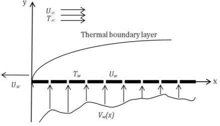
Let us suppose the existence of an incompressible power-law fluid with internal heat generation/absorption and all its physical properties assumed constant. The fluid flows over a porous plate with a sufficiently small injection/suction velocity that does not disturb the boundary layer assumption. The coordinate system is shown in Fig. 1.

Under these assumptions, the continuity and momentum equations are as follows:

Continuity: u v 0 x y  _ _

  (1)

Momentum:

 

1

yx

u u

u v

x x  y   _  _ 

   (2)

The boundary conditions for velocity are expressed as

w

u U v Vw

 

x _{at y} ₀

(3)

u U_ as y 

where Uw denotes the plate velocity in the negative x-direction, and U∞ represents the velocity of the uniform main stream.

H. Radnia / JHMTR 4 (2017) 53-64 55

For a power-law fluid, shear stress is given by

1 0 n yx u u y y      

  (4)

The energy equation with a heat

generation/absorption term is

2 2

p w

T T T Q T T

u v

x y  y C T T

 

   

  

    (5)

The fluid was analyzed only in the case wherein the temperature of the surface is kept constant (i.e., CST case). Accordingly, the thermal boundary conditions are

w

T T at y 0

(6) T T_ as y  

where Tw is the temperature at the plate surface, and

T∞ is the temperature outside the dynamic region.

3. Solutions of the Equations

A stream function is introduced to satisfy the continuity equation and to make the right hand side of the boundary condition (3) a constant value.

1 u L y     , 1 ( ) w

v V x

L x  

  

 (7)

The new variables are defined as:

Re

n x

L

  _{ }

 ,





  1 1

1 n y

n

L

_  _   _{ }

  (8)

where 2 0 Re n n U L      (9)

Re is the generalized Reynolds number. The stream function is also nondimensionalized through





1 1 ₂

 

1 n ,

n U L f

_  _  _  

(10) The momentum equation is eventually converted into [13, 14]







 







( 1) ,

1 ,

n f f

f f f f n 

 

  

      

 (11)

where the primes indicate partial differentiation with respect to η and









, ,

f f f f

f f

   



 _  _{ }

   (12)

is the Jacobian. Parameter Λ in Eq. (11) contains the injection velocity and is given by





( 1)

Re ( )

1 n n V

n n U

 _ 



  _  _ (13)

V() is defined as follows:

Re

( ) _w L

V V

n   _ _

  (14)

Note that if V(ξ) is negative, Λ will serve as the suction parameter.

The boundary conditions are converted into

w

U f

U_      

0

f  at0

(15) 1

f   As 

For the energy equation, the same method applied to momentum analysis is used. The dimensionless temperature is defined as

 

, w

w T T T T        (16)

The energy equation is then converted into







 

 



1 2 2 1

, 1

, f

f n 

   

 

           

 (17)

where the Jacobian is defined as,







,,



f f f   _      _ _{ }

   (18)

and





   





1 1 1 0 1 1 1 1 Pr 1 n n n n n U n n L x n n n

Here, Pr is the generalized Prandtl number, defined as

2 ( 1)

1

Pr Re n

U L     (20) and





2 2 1

2 1 n

p

Q L n

C 

  

  _  _ (21)

where Λ2 is the heat source/sink parameter.

The mathematical procedure of converting Eq. (5) into Eq. (17) is presented in Appendix 1. Dimensionless parameters Λ, Λ1, and Λ2 and variable

ξ are only the functions of x. These suggest the use of the Merk–Chao series to expand the solution in terms of these parameters.

Merk derived the momentum and energy boundary layer equations in transformed coordinates (ξ, η). He refined the “wedge method” by treating wedge parameter Λ, as an independent variable rather than stream wise coordinate ξ. Thus, the Merk series was expanded around the local similarity solution. As previously stated, Chao and Fagbenle put forward a corrected form of Merk’s series and used it to make a universal, laminar boundary layer analysis. Using the first term of the series can provide accurate results. The first term represents the local similarity solution, and the remaining terms enable a rigorous correction for departure from local similarity. Using the Merk– Chao series allows rapid calculations of boundary layer quantities with the aid of a limited number of universal functions [9, 15].

The dimensionless stream function is written as







 























0 1 2 2 2 2 2 2 2 2 3

, , , , 1 , ,

1 , ,

1 , ,

d

f n f n n f n

d d

n f n

d d

n f n

d                           _{ }    (22)

Subsequently, the dimensionless temperature is expanded as follows:

Incorporating Eqs. (22) and (23) into Eqs. (11) and (17) and collecting the terms containing similar perturbation quantities yield a set of sequential differential equations. The momentum equation is the same as that presented in [13].

The energy-related equations are





0 1 f0 0 2 0 2 0

        (24)













1 1 0 1 1 0 1 2 1

0 0

1 1 0 1 0 0

1

2

f n f

f

n f f

                     _        _  _  

  (25)









2 1 0 2 1 0 2

0 2 2 1 0

1

1

f n f

f                     (26)









3 1 0 3 1 0 3

0 2 3 1 0

2

1

f n f

f                     (27)

















4 1 0 4 1 0 4

2 4 1 0 2 1 1 0 0 1

2 1

2 3

f n f

n f f f

                  

       (28)









5 1 0 5 1 0 5

2 5 1 0 2

2 1

0

f n f

f               

    (29)









6 1 0 6 1 0 6

2 6 1 0 3

2 1

0

f n f

f               

    (30)

The boundary conditions are

0(0) 0

  0( ) 1

(31) (0) 0

i

  _i( ) 0 for i =

1,2,…,6

These equations, along with those for the momentum equation, generate a set of coupled first-order boundary value differential equations. To solve these equations, we adopted the fourth-order Runge– Kutta method, in which unknown initial values are obtained by applying the shooting method.

The shooting method is used to solve boundary value problems (BVP), with the approach involving the solution of initial value problems. A BVP is written in vector form, and the solution is carried out







 























0 1 1 2 2 3 2 2

2 2 2 2 1

4 5

2 2

2

2 2 2

6 2

, , , , 1

1 1

1 1

1

d

n n n

H. Radnia / JHMTR 4 (2017) 53-64 55

at one end of the BVP, after which this solution “shoots” to the other end with an initial value solver until the boundary condition at the other end converges to its correct value. An example is our solution for Eq. (24) with boundary conditions subject to θ0(0) = 0 and θ0(∞) = 1 (Eq. (31)). With the shooting method, θ0(0) = 0 is applied, along with a guess for θ0' (e.g., θ0' = a0). This method provides two initial conditions, thus enabling the application of the fourth-order Runge–Kutta method in solving this ordinary differential equation (ODE). The calculation proceeds until a value for θ0(∞) is obtained. If this does not satisfy θ0(∞) = 1 to an acceptable tolerance, the guess for θ0' is revised to a value a1, and the aforementioned method is repeated to obtain a new value for θ0(∞). This process continues until θ0(∞) = 1. Details regarding the application of the Runge–Kutta method in solving Eq. (24) are provided in Appendix 2.

The equations were solved with two different values of n: 0.52 for pseudoplastic (shear-thinning) fluids and 1.2 for dilatant (shear-thickening) fluids. The effects of a sink/source parameter (Λ2) on temperature profile were investigated on the basis of the values –0.5, 0, and 0.5. The surface velocity (λ) and Pr number were set at 0.1 and 7, respectively, where injection/suction velocity (Λ) varies between – 1.5 and 0.3.

The unknown initial conditions for the momentum equation are the same as those indicated in previous work [14]. Therefore, the numerical results of that work were applied in the current research (Table 1). The results with respect to the unknown initial conditions for the energy equations are presented in Tables 2 and 3.

The simplest case for this problem is when the injection parameter is a constant, where



n 1



d n

d

 



   (32)





2 2 2 2

1 d

n n

d

 



    (33)





1





1

1 d 1

n n

d

 



    ₍₃₄₎





2 2 2 1





1 2

1 d 2 1

n n n

d

 



     (35)





2





2

1 d 1

n n

d

 



    ₍₃₆₎





2 2 2 2





2 2

1 d 2 1

n n n

d

 



     (37)

Applying the same procedure as explained by Rao et al. [13], we obtained nondimensionalized temperature profiles under different conditions.

Table 1. Numerical results of fi"(0) for n = 0.52 and 1.2 [13].

n = 0.52 n = 1.2

  f₀ f₁

f

₂



f

₀



f1

f

2



0.1

-1.5 1.209760 0.079552 -0.011380 1.375745 0.082688 -0.01192 -0.75 0.645513 0.068450 -0.010755 0.702922 0.068498 -0.01091 0 0.286023 0.050589 -0.008666 0.279605 0.045026 -0.00795 0.3 0.191973 0.042005 -0.007423 0.171299 0.032493 -0.00608 Table 2. Numerical results of θ0'(0) for n = 0.52, Λ1 = 1.633 (corresponding to Pr = 7 and x/L = 0.1), and λ = 0.1.

2 

0(0)





1(0)



2(0) 3(0)



4(0) 5(0) 6(0)

-0.5

-1.5 2.6637 _{0.22536 -0.04986 0.06901 -0.0156 0.00483 -0.0068} -0.75 1.615 _{0.26165 -0.0472 0.06259 -0.0193 0.00559 -0.0072} 0 0.75058 _{0.22909 -0.0219 0.04272 -0.01719 0.00322 -0.0058} 0.3 0.51839 0.16398 -0.03044 0.0468 -0.02548 0.00587 -0.00909

0

-1.5 2.5032 _{0.0458 -0.0776 0.0558 -0.0012 0.0113 0.0038} -0.75 1.3762 0.0851 -0.0685 0.0621 -0.0071 0.0136 -0.0069

0 0.39263 _{0.13299 -0.0211 0.0431 -0.02156 0.00843 -0.0055} 0.3 0.14095 0.09714 -0.00123 0.02318 -0.0171 0.00378 -0.00159

0.5

-1.5 2.325 0.3579 0.0306 0.09206 -0.0265 0.00803 -0.00558 -0.75 1.0764 _{0.393645 -0.0452 0.08551 -0.03039 0.00879 -0.00599} 0 -0.2596 0.36103 -0.00912 0.06572 0.02819 0.00642 -0.0045 0.3 -0.7278

Table 3. Numerical results of θ0'(0) for n = 1.2, Λ1 = 1.633 (corresponding to Pr = 7 and x/L = 0.1), and λ = 0.1.

2 

0(0)





1(0)



2(0)



3(0)



4(0)



5(0)



6(0)

-0.5

-1.5 2.677

0.0385 -0.0765 0.0594 -0.0021 0.0098 -0.0037 -0.75 1.61445 0.06148 -0.0652 0.06903 -0.0078 0.01126 -0.00725

0 0.74826 0.05218 -0.01704 0.03448 -0.02381 0.00487 0.00435 0.3 0.521574 0.017268 -0.006195 0.03645 -0.01829 -0.00108 -0.00436

0

-1.5 2.5187

0.0394 -0.0757 0.0355 -0.0031 0.00752 -0.00771 -0.75 1.3732 0.0709 -0.0664 0.0313 -0.0094 0.01725 -0.00997 0 0.38644 0.12018 -0.01413 0.02147 -0.0354 0.00453 -0.00746 0.3 0.15433 0.07237 -0.00136 0.01748 -0.0301 0.00078 -0.00549

0.5

-1.5 2.344

0.2433 0.0506 0.0736 -0.01685 0.00553 -0.0054 -0.75 1.067 0.27645 -0.0812 0.0691 -0.02059 0.006299 0.0095

0 -0.2952 0.24039 -0.02269 0.047402 0.01839 0.003922 -0.00546 0.3 -0.5912 0.18918 -0.0324 0.05088 -0.02668 0.00687 -0.0085

4. Results and Discussion

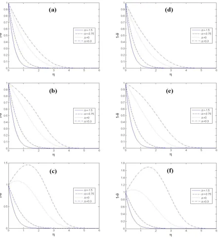
The effects of power n on a

nondimensionalized temperature profile are illustrated in Fig. 2. Note that in all figures,

1 w

T T

T T

 

   



is plotted against η. The results

revealed that the thickness of the temperature boundary layer decreases with increasing n. In other words, the boundary layer of a shear-thinning power-law fluid (n < 1) is more expansive than that of a shear-thickening power-law fluid (n > 1). This difference is more significant in the presence of heat generation. These results accord with those of previous works [12–14]. That is, an increase in n

leads to an augmentation in heat transfer [16]. The nondimensionalized temperature profiles at different values of injection/suction and heat source/sink parameters and two values of n are shown in Fig. 3. The thickness of the thermal boundary layer decreases when a suction flow exists (Λ<0), as is evident in Fig. 3. The fluid is brought closer to the wall, thereby reducing the thickness of the thermal boundary layer. This reduction decreases the temperature profiles. The temperature decreases to a greater extent as the suction parameter increases, indicating that increased suction leads to faster surface cooling. However, the exact opposite behavior is produced by the injection of a fluid onto the surface (Λ>0). Injection generates more flow penetration into the fluid, which causes an increase in the thermal boundary layer. The effects of suction/injection parameters were also investigated in the literature [8, 17].

The main concern here are the effects of a heat source/sink parameter (Λ2) on temperature profile. Fluid temperature is greater when internal energy is generated (Λ2>0), which drives a thickness increase in the thermal boundary layer (Fig. 3). This result is expected given that the presence of a heat source in the boundary layer generates energy and thus increases the temperature of the fluid, leading to an increase in the thickness of the thermal boundary layer. Contrastingly, the heat sink (Λ2<0) exerts an opposite effect on the thickness of the thermal boundary layer. Specifically, it causes a drop in temperature and reduces the thickness of the thermal boundary layer. These effects have been discussed in previous researches [4, 5].

Note that in the presence of heat generation (Fig.s 2-c and 2-f), during which no suction/injection (Λ = 0) exists, the maximum fluid temperature does not occur at the wall but in the fluid region close to it. A peak in temperature profile occurs in the fluid near the wall, indicating that the temperature of the fluid near the sheet is higher than that of the sheet. In other words, heat is transferred from the fluid to the wall. This peak is sharper when the injection parameter used is Λ>0. The same trend does not occur in the presence of a suction parameter because, as previously mentioned, suction contributes to surface cooling.

H. Radnia / JHMTR 4 (2017) 53-64 55

the surface. The authors transformed the resultant governing equations into nonlinear ODEs by using appropriate transformations and then numerically solved the ODEs on the basis of central difference approximations. Abo-Eldahab et al. [19] delved into heat transfer through mixed convection along an inclined continuously stretching surface under internal heat generation/absorption. The authors regarded the surface as permeable to allow fluid suction or blowing and stretching with surface velocity. They converted the governing equations into dissimilar partial differential equations (PDEs), which they then integrated using the fourth-order Runge–Kutta method. Mahmoud and Megahed [20] examined the effects of non-uniform heat generation/absorption and viscous dissipation on the heat transfer of a non-Newtonian power-law fluid flowing on a nonlinearly stretching surface. The authors converted the governing nonlinear PDEs into a system of nonlinear ODEs by using suitable similarity transformation. The researchers then numerically solved the ODEs by using the fourth-order Runge–Kutta method combined with the shooting technique. A comparison of these numerical methods with the approach used in the present study reflected a difference in procedures for converting PDEs into ODEs. In our study, the Merk–Chao series was used for this transformation. The Merk–Chao series expansion is a useful method for solving difficult transport problems in simple transformations. Universal functions are used to solve fundamental differential equations, regardless of geometry.

5. Conclusion

The problem of the boundary layer heat transfer of a non-Newtonian power-law fluid flowing on a

porous moving surface under heat

generation/absorption was studied. The governing equations describing the problem were converted into a set of ODEs by using the Merk–Chao series. The ODEs were then solved numerically by adopting the fourth-order Runge–Kutta method, coupled with the shooting technique. The effects of different parameters on dimensionless temperature were illuminated with respect to constant velocity at

the plate surface. The results indicated that the thermal boundary layers of pseudoplastic fluids are thicker than those of dilatants. A direct relationship exists between dimensionless temperature and an increase in injection or heat generation parameters.

Fig. 2.Effects of fluid types (dilatant fluid with n = 0.52 and pseudoplastic fluid with n = 1.2) on temperature profile: λ = 0.1, Λ1 = 1.633, Λ = 0.3 for a, b, and c at Λ2 = –

0.5, 0, and 0.5, respectively.

Fig. 3. Effects of injection/suction and heat source/sink on temperature profile for two different cases: n = 1.2, λ = 0.1, Λ1 =

1.633 for a, b, and c at Λ2 = –0.5, 0, and 0.5, respectively; n = 0.52, λ = 0.1, Λ1 = 1.633 for d, e, and f at Λ2 = –0.5, 0, and 0.5,

respectively.

Nomenclature

Cp Specific heat at constant pressure

f Dimensionless stream function defined in Eq.

(10)

k Thermal conductivity

L Reference length

n Power-law exponent defined in Eq. (4)

Pr Generalized Prandtl number defined in Eq. (20)

Q Volumetric rate of heat generation

Re Generalized Reynolds number defined in Eq. (9)

T Temperature

u Fluid velocity component in the x-direction

Uw Plate velocity in the negative x-direction

U∞ Main stream velocity

v Fluid velocity component in the y-direction

ν0 Constant injection velocity at the wall

Vw Injection velocity at the plate surface

54 H. Radnia / JHMTR 4 (2017) 53-64

x Stream-wise coordinate along the surface measured from the slot

y Coordinate normal to the plate surface

Greek symbols

α Thermal diffusivity

η Dimensionless variable defined in Eq. (8)

θ Dimensionless temperature defined in Eq. (16)

λ Plate velocity ratio defined in Eq. (15)

Λ Injection parameter defined in Eq. (13)

Λ1 Parameter in the energy equation defined in Eq. (19)

Λ2 Heat source/sink parameter defined in Eq. (21)

µ0 Consistency index for non-Newtonian viscosity defined in Eq. (4)

ξ Dimensionless variable defined in Eq. (8)

ρ Density

τxy Shear stress defined in Eq. (4)

ψ Stream function defined in Eq. (7)

Subscripts

i Subscript designating universal functions

w Subscript designating conditions at the plate surface

∞ Subscript designating conditions in the main stream

Reference

[1].L. Deswita, A. Ishak, R. Nazar, "Power-Law Fluid Flow on a Moving Wall with Suction and Injection Effects", Australian Journal of Basic and Applied Sciences, 4 (8), (2010) pp. 2250-6.

[2].R. Cortell, "Suction, Viscous Dissipation and Thermal Radiation Effects on the Flow and Heat Transfer of a Power-Law Fluid Past an Infinite Porous Plate", Chemical Engineering Research and Design, 89 (1), (2011) pp. 85-93.

[3].W. Schowalter, "The Application of Boundary-Layer Theory to Power-Law Pseudoplastic Fluids: Similar Solutions", AIChE Journal, 6 (1), (1960) pp. 24-8.

[4].E.M. Abo-Eldahab , M.A. El Aziz, "Blowing/Suction Effect on Hydromagnetic Heat Transfer by Mixed Convection from an Inclined Continuously Stretching Surface with Internal Heat Generation/Absorption", International Journal of Thermal Sciences, 43 (7), (2004) pp. 709-19. [5].M.A. Mahmoud, "Slip Velocity Effect on a Non-Newtonian Power-Law Fluid over a Moving Permeable Surface with Heat Generation",

Mathematical and Computer Modelling, 54 (5), (2011) pp. 1228-37.

[6].M. Seddeek, "Finite-Element Method for the Effects of Chemical Reaction, Variable Viscosity, Thermophoresis and Heat Generation/Absorption on a Boundary-Layer Hydromagnetic Flow with Heat and Mass Transfer over a Heat Surface", Acta Mechanica, 177 (1-4), (2005) pp. 1-18.

[7].M.S. Abel, P. Siddheshwar, M.M. Nandeppanavar, "Heat Transfer in a Viscoelastic Boundary Layer Flow over a Stretching Sheet with Viscous Dissipation and Non-Uniform Heat Source", International Journal of Heat and Mass Transfer, 50 (5), (2007) pp. 960-6.

[8].R. Cortell, "Flow and Heat Transfer of a Fluid through a Porous Medium over a Stretching Surface with Internal Heat Generation/Absorption and Suction/Blowing", Fluid Dynamics Research, 37 (4), (2005) pp. 231-45.

[9].F. Lin , S. Chern, "Laminar Boundary-Layer Flow of Non-Newtonian Fluid", International journal of heat and mass transfer, 22 (10), (1979) pp. 1323-9.

[10].H. Kim, D. Jeng, K. DeWitt, "Momentum and Heat Transfer in Power-Law Fluid Flow over Two-Dimensional or Axisymmetrical Bodies", International journal of heat and mass transfer, 26 (2), (1983) pp. 245-59.

[11].C. Tien-Chen Allen, D.R. Jeng, K.J. DeWitt, "Natural Convection to Power-Law Fluids from Two-Dimensional or Axisymmetric Bodies of Arbitrary Contour", International journal of heat and mass transfer, 31 (3), (1988) pp. 615-24. [12].A. Sahu, M. Mathur, P. Chaturani, S.S. Bharatiya, "Momentum and Heat Transfer from a Continuous Moving Surface to a Power-Law Fluid", Acta Mechanica, 142 (1-4), (2000) pp. 119-31.

[13].J. Rao, D. Jeng, K.D. Witt, "Momentum and Heat Transfer in a Power-Law Fluid with Arbitrary Injection/Suction at a Moving Wall", International Journal of Heat and Mass Transfer, 42 (15), (1999) pp. 2837-47.

[14].H. Shokouhmand , M. Soleimani, "The Effect of Viscous Dissipation on Temperature Profile of a Power-Law Fluid Flow over a Moving Surface with Arbitrary Injection/Suction", Energy Conversion and Management, 52 (1), (2011) pp. 171-9.

[15].A. Falana , R.O. Fagbenle, "Forced Convection Thermal Boundary Layer Transfer for Non-Isothermal Surfaces Using the Modified Merk Series", Open Journal of Fluid Dynamics, 4 (02), (2014) pp. 241.

[16].A. Tamayol, K. Hooman, M. Bahrami, "Thermal Analysis of Flow in a Porous Medium over a Permeable Stretching Wall", Transport in Porous Media, 85 (3), (2010) pp. 661-76.

[17].G. Layek, S. Mukhopadhyay, S.A. Samad, "Heat and Mass Transfer Analysis for Boundary Layer Stagnation-Point Flow Towards a Heated Porous Stretching Sheet with Heat Absorption/Generation and Suction/Blowing", International Communications in Heat and Mass Transfer, 34 (3), (2007) pp. 347-56.

[18].C.-H. Chen, "Effects of Magnetic Field and Suction/Injection on Convection Heat Transfer of Non-Newtonian Law Fluids Past a Power-Law Stretched Sheet with Surface Heat Flux", International journal of thermal sciences, 47 (7), (2008) pp. 954-61.

[19].E.M. Abo-Eldahab, M.A. El-Aziz, A.M. Salem, K.K. Jaber, "Hall Current Effect on Mhd Mixed Convection Flow from an Inclined Continuously Stretching Surface with Blowing/Suction and Internal Heat Generation/Absorption", Applied Mathematical Modelling, 31 (9), (2007) pp. 1829-46.

[20].M.A. Mahmoud , A.M. Megahed, "Non-Uniform Heat Generation Effect on Heat Transfer of a Newtonian Power-Law Fluid over a Non-Linearly Stretching Sheet", Meccanica, 47 (5), (2012) pp. 1131-9.

Appendix 1. Converting Eq. (5) into Eq. (17)

Eq. (16) is used to convert variable T to dimensionless form (θ) in Eq. (5). Thus, the energy equation is eventually transformed into

2

2 ( 1)

p

Q

u v

x y y C

  _  _



  

   

   (A1.1)

θ is assumed to be a function of ξ and η (Eq. (16)), which are defined in Eq. (8). Thus,   x ,   y, and 2 2

y



  can be derived as follows:

( ) ( )

Re 1 Re

n n

x x x L n L

       

    

       

   

        _(A1.2)

1 1

[( 1) ]

( )

n

n

y y y L

      

  

 

 _  _  _  

      (A1.3)

2

2 1 2

2 2 2

[( 1) ]

( ) ( )

n

n

y y y L

   



 

 _   _  

    (A1.4)

According to the definition of ψ (Eq. (10)),   x

and  y are derived thus:

1

[( 1) ] [ ( 1) ]

Re

n n

nU f f

n f n

x L  _{  }       _{    }  _ 

   (A1.5)

f U L y     _ 

  (A1.6)

The following equations are derived for u and v by substituting Eqs. (A1.5) and (A1.6) into Eq. (7):

1

[( 1) ] Re

Re

[ ( 1) ] ( )

n n

w

nU

v n

f f L

f n V

n                      (A1.7) f u U      (A1.8)

Substituting Eqs. (A1.2), (A1.3), (A1.4), (A1.7), and (A1.8) into Eq. (A1.1) and simplifying the energy equation yield

                  1 1 1 0 2 2 ( 1)

2 2 2 2

1 1

1

1 1

0

1

Re ( ) 1 1 1 1 ( n n n n n n n p p n n n U n n L V f n n U

Q L Q L

n n C C U n n L n  _     _           _               _{ }      _  _    _{ } _  _{   } _  _  _{ }                                  _{ }      _  _      

 1) 

f f              _     _{   } _  _    (A1.9)

Eq. (A1.9) can be overwritten to establish Eq. (17).







 

 



1 2 2 1

, 1

, f

f n 

   

             

 (17)

Here, the primes are defined as partial differentiations with respect to η. Λ, Λ1, and Λ2 are defined in Eqs. (13), (19), and (21); the term

,f   ,

  is Jacobian and defined in Eq. (18) in the main text.

Appendix 2. Numerical Procedure

54 H. Radnia / JHMTR 4 (2017) 53-64

term of the Merk–Chao series for the energy equation. This equation, along with the momentum equation, generates a set of coupled first-order boundary value differential equations. The first term of the Merk–Chao series for the momentum equation is

 

1





0

''' '' ''

0 0 0 0

n

f f   f   f  (A2.1)

Eq. (A2.1) and the other terms of the Merk– Chao series for the momentum equation can be found in the paper published by Rao et al. [13].

To solve these equations, the fourth-order Runge–Kutta method is adopted. The third-order ODE of the momentum equation can be converted into a system of three first-order ODEs through the following variable substitution:





0 0 0 0 0 0 1 0 0 ' 0 '' 0 ''' 0 n f y f z f u y u f q u           (A2.2)

The same substitution procedure is used to convert the second-order ODE of the energy equation (Eq. (24)) into a system of two first-order ODEs as follows:





0 0

0 0

0 0 1 0 0 2 0 2

r s

t y s r

                  (A2.3)

These ODEs are solved in the interval 0 ≤ x ≤ 8 by using 80 intervals (i.e., with h = 0.1) as follows:

 





0 0 01 1 0 01 0 01 0

01 1 0 0 2 0 2

01 0 ( ) n y u K h u

L h z

M h u

N h y s r

O h s

                            (A2.4) 01 01 0 0 02 1 01 0 01 02 0 01 02 0 01 01

1 0 0

02

01

2 0 2

01 02 0 2 2 2 2 2 2 2 2 2 n L K y u K h K u M

L h z

K

M h u

L N y s N h O r N

O h s

 _ _ _{  }  _  _ _ _ _ _ _      _    _ _       _  _    _  _ _ _ _{  }  _ _  __ _ _ _ _     _{ }         _ _       _  _ (A2.5) 02 02 0 0 03 1 02 0 02 03 0 02 03 0 02 1 0 03 02 02

0 2 0 2

02 03 0 2 2 2 2 2 2 2 2 2 n L K y u K h K u M

L h z

K

M h u

L y N h N O s r N

O h s

 _ _ _{  }  _  _ _ _ _ _ _     _{ }    _ _       _  _      _  _   _  _ _{  }   __ _ _      _{   }         _ _ _ _       _    (A2.6) 03 03 0 0 04 1 03 0 03 04 0 03 04 0 03 1 0 04 03 03

0 2 0 2

03 04 0 2 2 2 2 2 2 2 2 2 n L K y u K h K u M

L h z

K

M h u

L y N h N O s r N

O h s

 _ _ _{  }  _  _ _ _ _ _ _     _{ }    _ _       _  _      _  _   _  _ _{  }   __ _ _     _{ }  _ _{  } _ _{ } _ _ _ _       _    (A2.7) Finally,    

01 02 03 04

0 0

01 02 03 04

0 0

01 02 03 04

0 0

0 0

0 1

0

01 02 03 04

0 0

01 02 03 04

0 0

0 1 0 0 2 0 2

2 2 6 2 2 6 2 2 6 2 2 6 2 2 6 n

L L L L

y y

M M M M

z z

K K K K

u u

y u

q

u

N N N N

s s

O O O O

r r

t y s r

       _{  }         _{  }         _{  }              _{  }         _{  }             (A2.8)

Because Eqs. (24) and (A2.1) are BVPs, the shooting method is used to solve the problem, as described in the main text. For this purpose, si0 is modified as the problem is run until t(∞) = 1 or 1-t(∞) = 0 is achieved. This procedure is carried out using MATLAB (R2007a). The same procedure is used for Eqs. (25) to (30), and the results for different values of n, Λ, and Λ1 are listed in Tables 2 and 3. Note that the momentum equation was previously solved by Rao et al. [13], and we used their results, as presented in Table 1.