Bayesian estimation of parameters in a regional hydrological
model
Kolbjørn Engeland
1and Lars Gottschalk
21Norwegian Water Resources and Energy Directorate, P.O. Box 5091,Majorstua, 0301 Oslo, Norway 2Department of Geophysics, University of Oslo, P.O. Box 1022 Blindern, 0315 Oslo, Norway
Email of corresponding author: kolbjørn@engeland.no
Abstract
This study evaluates the applicability of the distributed, process-oriented Ecomag model for prediction of daily streamflow in ungauged basins. The Ecomag model is applied as a regional model to nine catchments in the NOPEX area, using Bayesian statistics to estimate the posterior distribution of the model parameters conditioned on the observed streamflow. The distribution is calculated by Markov Chain Monte Carlo (MCMC) analysis. The Bayesian method requires formulation of a likelihood function for the parameters and three alternative formulations are used. The first is a subjectively chosen objective function that describes the goodness of fit between the simulated and observed streamflow, as defined in the GLUE framework. The second and third formulations are more statistically correct likelihood models that describe the simulation errors. The full statistical likelihood model describes the simulation errors as an AR(1) process, whereas the simple model excludes the auto-regressive part. The statistical parameters depend on the catchments and the hydrological processes and the statistical and the hydrological parameters are estimated simultaneously. The results show that the simple likelihood model gives the most robust parameter estimates. The simulation error may be explained to a large extent by the catchment characteristics and climatic conditions, so it is possible to transfer knowledge about them to ungauged catchments. The statistical models for the simulation errors indicate that structural errors in the model are more important than parameter uncertainties.
Keywords: regional hydrological model, model uncertainty, Bayesian analysis, Markov Chain Monte Carlo analysis
Introduction
BACKGROUND
Regional hydrological modelling enables a solution of a classical problem in hydrology, namely the estimation of the water balance in ungauged catchments. This implies repeated use of a model everywhere within a region using a global set of parameters. Use of regional parameters in streamflow simulations for individual catchments results in some loss of precision (Motovilov et al., 1999). The obvious gain is in the ability to calculate runoff in ungauged basins but more robust model parameters and a smaller parameter uncertainty also result (Engeland et al., 2001). Regionalisation methods search for a relationship between model parameters and landscape characteristics. While for lumped models, multiple regression between model parameters and catchment characteristics can be used (e.g. Abdulla and Lettenmaier, 1997), for distributed models the
UNCERTAINTIES IN HYDROLOGICAL MODELLING
Neither the regression method nor the proxy basin test accounts for the uncertainties in the hydrological modelling. To know how well the model performs in a regional application, the modelling uncertainties have to be identified and quantified. The simulation errors of a hydrological model have four important sources (Refsgaard and Storm, 1996):
(1) random or systematic errors in input data, i.e. precipitation, temperature and evapotranspiration, etc. used to represent the input conditions in time and space over the catchment;
(2) random or systematic errors in the recorded data, i.e. the river water levels, groundwater heads, discharge data or other data used for comparison with the simulated output;
(3) errors due to non-optimal parameter values; (4) errors due to incomplete or biased model structure.
Error sources (1) and (2) depend on the quality of the data whereas (3) and (4) are more model-specific. In several papers, two or more of the error sources are included in the estimation of the total modelling uncertainty. Thorsen et al. (2001), Refsgaard et al. (1983) and Storm et al. (1988) conclude that the uncertainty in precipitation is more important than that in the parameters. Krzysztofowicz (1999) shows that, in hydrological forecasts, the uncertainties in the precipitation forecasts are more important than those in the hydrological model. For regional studies, the importance of model and parameter uncertainties might increase, so it is the parameter and model uncertainties that are investigated in this paper.
Of several tools developed to investigate the uncertainties in hydrological models, at least two might be used for regionalisation. The multi-objective method of Gupta et al. (1998) cautions that there might not exist any correct objective function that adjusts the simulated streamflow to all parts of the observed record, e.g. timing and magnitude of flood peaks, the recession after high flows, low flows and the water balance. The multi-objective method, therefore, estimates a parameter uncertainty due to the trade-off between different objective functions and might be used for regionalisation by estimating the uncertainty due to the trade-off between the objective function for several catchments. Another possibility is the Bayesian method (Kuzcera, 1983), which is applied in this paper. The Bayesian method estimates a probability density for the model parameters conditioned on observations. The uncertainty is calculated around the optimal value of one
objective function. Beven and Binley (1992) introduced a variant of this method known by the acronym GLUE (Generalised Likelihood Uncertainty Estimation). The Bayesian method requires a likelihood function that describes the statistical properties of the simulation errors, whereas in the GLUE framework any subjectively chosen objective function might be used as the likelihood.
OBJECTIVES
This study evaluates the applicability of the distributed process-oriented Ecomag model (Motovilov et al., 1999) for prediction of streamflow in ungauged basins in the experimental area of the NOrthern hemisphere climate-Processes land-surface EXperiment (NOPEX) (Halldin et al., 1995; 1999). To be suitable for regional applications, a hydrological model should fulfil the following requirements:
z the model results should be robust;
z the regional model parameter should be well defined; z the statistical model for the simulation errors should be
transferable to ungauged catchments.
The first requirement might be tested by a cross-validation test. Motovilov et al. (1999) used the proxy-basin test with good results for the Ecomag model adapted to the NOPEX area. Furthermore, Engeland et al. (2001) concluded that well defined regional parameters can be determined according to pre-defined criteria. The GLUE concept showed that the variance of the parameter distribution decreased as streamflow observations from several catchments were included in the parameter estimation.
should perform well on average but the variation in performance between catchments should be small. The performance measure is the Nash-Sutcliffe coefficient Reff (Nash and Sutcliffe, 1970). The transferability of the simulation errors will be tested. If the simulation errors are transferable, it should be possible to relate them to catchment characteristics or climatic conditions.
Data and model description
THE NOPEX AREA
The NOPEX project (Halldin et al., 1995; 1999) established a study area in southern Sweden, northwest of Uppsala in an area of low relief where the altitude ranges from 5 to 145 m.a.s.l. Till is the most common soil type, particularly in the north. Clay soils with sandy and silty materials dominate in the south while, in the north, peat covers the largest area. (Seibert, 1994). The important land use classes are forests (57%), mires (2.6%), lakes (2.6%) and urban areas (2.0%). The average annual precipitation is 740 mm, evapo-transpiration 470 mm, and runoff 270 mm. The area is covered by snow for about 110 days a year but the snow cover is normally not continuous throughout the winter. The
mean annual temperature is +6oC, with a maximum in July
(+17oC) and a minimum in February (–5oC). The vegetation
period lasts about 180 days (Seibert, 1994).
METEOROLOGICAL AND HYDROLOGICAL DATA
The data are provided from the SINOP (System for Information in NOPex) database (Lundin et al., 1999) developed in the NOPEX project. The Swedish Meteorological and Hydrological Institute (SMHI) provides daily values from 25 precipitation, 7 temperature, 5 air humidity, and 10 streamflow stations for the period from 1981–1990. All stations are located within or close to the NOPEX area. The gauged catchments cover a large part of the area (Fig. 1). Short catchment descriptions are given in Table 1.
THE ECOMAG MODEL
The Ecomag model (Motovilov et al., 1999) calculates streamflow Qi,t,sim (θθθθθ,D[t-t’,t]) on a daily time resolution as a function of model parameters θθθθθ and input data D (D is precipitation, air temperature and vapour pressure deficit, i is an index for catchment, t an index for time, and t’ is the
[image:3.595.89.533.407.703.2]length of the memory of the hydrological model). The model area is divided into grid cells and the same process formulations are applied within each cell independently. A threshold temperature decides the phase of precipitation. Snow melt is estimated by a degree-day-factor equation, evapotranspiration by Thornthwaite-Budyko, surface runoff by a kinematic wave formulation, horizontal subsurface flow
by Darcy’s law and vertical movement is controlled by the infiltration capacity. The point input observations are interpolated to each grid cell by the inverse distance weighting method. The vertical structure of a grid cell is shown in Fig. 2.
[image:4.595.45.544.89.256.2]Each grid cell is assigned the soil and vegetation class covering most of its respective area. Some of the parameters Table 1. Characteristics for gauged catchments in the NOPEX area.
No Station Catchment Area (km2) Lake (%) Forest (%) Open land(%)
1 Ulva Kvarndamn Fyrisån 950.0 3.0 61.0 36.0
2 Sörsätra Sagån 612.0 1.1 61.0 37.9
3 Gränvad Lillån 168.0 0.0 41.0 59.0
4 Härnevi Örsundaån 305.0 1.0 55.0 44.0
5 Lurbo Hågaån 124.0 0.3 77.7 27.0
6 Ransta Sävaån 198.0 0.9 66.1 33.0
7 Sävja Sävjaån 727.0 2.0 64.0 34.0
8 Tärnsjö Stalbobäcken 14.0 1.5 84.5 14.0
9 Stabby Stabbybäcken 6.6 0.0 87.0 13.0
10 Vattholma Fyrsiån 284.0 - -
-R iver flo w
p recip itation
sur face w a te r sto rage surfac e w ater outflow
subsurfa ce outflow horizon A
subsurfa ce outflow horizon B
groundw ate r out flow ice particles
field cap a city W P
E4
surface w a ter inflow
subsurfa ce inflow horizon A
subsurfa ce inflow horizon B
groundw ate r inflow
p o ro sit y
s
l i o
s
l i o
i m
r t a
x i m
r t a
x
gr oun dw ater zo ne h ori zo n B
h4
e
v
a
p
ot
ra
n
s
p
ir
a
ti
on
melt water sno w cover
horizon A
in
filt
ra
tion
re
tu
rn
fl
o
w
p
ene
trat
io
n
p
e
ne
trat
io
n
h3
Z4
h2
Z2
Z3
ca pilla ry zo ne
no n zo ne ca pilla ry
in
filt
ra
tio
n
h1 h5
no n z one ca pilla ry ca pilla ry
zo ne
E5
E1
E2
E3
[image:4.595.76.510.370.711.2]in θθθθθ depend on the soil or vegetation class of the grid cell, whereas the remaining parameters are common for the whole region. The parameters that depend on the soil and vegetation classes are not calibrated for each individual class but the standard parameter values are multiplied by a common factor. For each parameter, the relative differences between its value for the soil or vegetation classes are determined prior to the calibration. This procedure reduces the number of parameters that need to be calibrated.
APPLICATION OF ECOMAG TO THE NOPEX AREA
The chosen grid-size is 2 × 2 km. As the average slope length is less than 2 km, subsurface flow between grid cells is omitted. The water is assumed to flow directly into the river. As few geographical data are available for the Vattholma catchment, streamflow at Vattholma is included in the model for calculating streamflow at Ulva Kvarndam further downstream (Fig. 1). Six soil classes (till, clay, sand, peat, shallow bedrock, and lake) and five land-use classes (forest, open, peat, and lakes) are defined.
The present study is based on Motovilov et al. (1999) in which, following the proxy basin test (Klemeš, 1986), a regional calibration and validation of Ecomag was performed as well as validation of internal variables. As a first step, the model was calibrated using 7 years’ streamflow data for three catchments. The soil parameters were adjusted using soil moisture and groundwater data from five small experimental catchments. Thereafter, the model was validated against 14 years’ streamflow measurements from six other catchments as well as synoptic streamflow and evapotranspiration measurements during two concentrated field efforts in 1994 and 1995.
The nine parameters that were the most sensitive to simulation of streamflow are included in the MCMC simulations. They are: vertical conductivity of horizon A, horizontal conductivity of horizon A, horizontal conductivity of the groundwater zone, thickness of horizon A, evaporation, surface depression storage, degree-day-factor, critical temperature of snow/rain precipitation, and the threshold temperature for start of snowmelt. The first four parameters depend on soil class, the following three on the land-use class, while the last two are common for the whole area.
The Bayesian method
The Bayesian method estimates a multi-dimensional probability density p(θθθθθ,ϕϕϕϕϕ|Y) for the hydrological parameters θθθθθ and the statistical parameters ϕϕϕϕϕ conditioned on the streamflow observations Y:
(
) (
p C)
p( )
pθ,φY = Yθ,φ θ,φ (1)
where p(θθθθθ,ϕϕϕϕϕ) is the prior density and C is a normalisation constant. When the data Y are given, p(Y|θθθθθ,ϕϕϕϕϕ) might be regarded as a function of θθθθθ and ϕϕϕϕϕ which is the likelihood function of θθθθθ and ϕϕϕϕϕ given Y and is written L(θθθθθ,ϕϕϕϕϕ|Y). Hence:
(
) (
L C)
p( )
pθ,φY = θ,φY θ,φ (2)
Due to non-linearities in the model, the probability density may have an irregular surface containing several local maxima and therefore be far from normally distributed. The density is, therefore, simulated by MCMC.
FORMULATION OF THE LIKELIHOOD FUNCTION
The formulation of the likelihood function L(θθθθθ,ϕϕϕϕϕ|Y) controls the probability distribution of the parameters (Boyle et al., 2000). The likelihood is proportional to the probability of the vector of simulation errors δδδδδ that is the differences between observed and simulated streamflows:
(
θ φY) (
f δθ,φ)
L , ∝ (3)
where f is any multidimensional probability density function. The statistical properties of the simulation errors have to be investigated carefully. The simulation errors might depend on the catchment or the hydrological processes and they might be correlated both in time and space. Kuczera (1983), Sorooshian (1991), Romanowicz et al. (1994), Langsrud et al. (1998) and Engeland (2002) among others have constructed statistical models for the simulation error that take into account one or more of these aspects. To find a suitable likelihood function is difficult. Gupta et al. (1998) suggested that no objective and statistically correct likelihood-function might exist. No study, as far the authors know, includes the spatial dependence of the simulation errors. The full space-time structure of the simulation errors is difficult to grasp for a hydrological model operating on daily time steps. The structure will, amongst others, depend on the relative differences between the catchment responses. In this study, the auto-correlations are accounted for whereas the spatial correlations are not included.
[
itobs]
[
itsim(
ttt)
]
t
i, =logQ,, −logQ,, θ,D−,'
δ (4)
Two models for the simulation errors are constructed. The simple model is contained within the full one, so the full model is presented. The simulation errors are modelled as an AR(1) process where the parameters depend on the hydrological processes and the catchments:
( )
(
i kit)
(
k( )it i)
(
it(
i k(it ))
)
it ti, µ m , α , β δ, 1 µ m , 1 ε,
δ − + = + − − + − +
(
(,))
,t ~ 0, i kit
i N ω τ
ε + (5)
where i is an index (i = 1,...,9) for the nine first catchments listed in Table 1, and k(i,t) is an index function (k = 1,...,13) for the climate classes listed in Table 2. The climate class for catchment i at time t is decided by the average precipitation and temperature at time t within each catchment in addition to the observed snow depth at one location. The climate classes are chosen to distinguish between important hydrological processes. The simulation errors are assumed to be different for increasing runoff compared to recession periods. The rate of evapotranspiration might be important for the recession and low flows, whereas snow melt and rain decide the high flows. It is necessary to take special care of the snow accumulation and snow melt processes because they make the hydrological system extremely non-linear. Based on these considerations, the climate is classified into temperature intervals, and each temperature class is divided into four subclasses dependent on the possible combinations of observed precipitation and observed
snow-cover. This parameterisation combines information about the simulation errors across the catchments. The climate-dependent parameters will show whether it is possible to transfer information about the simulation errors to ungauged catchments. For the bias and the variance parameters, climate class 13 is chosen as a reference (m13=0, τ13=0). The Fyrisån
catchment is chosen as a reference for the auto-regressive parameters (β1=0). Positively biased parameters indicate
under-estimation and negative values indicate over-estimation of streamflow. Using this parameterisation, the mk and ωk parameters will adjust the bias and variance to
each climate class, whereas βi will adjust the auto-correlation
to each catchment. The total number of parameters to be estimated for the full model is 72: 21 location parameters, 21 auto-regressive parameters and 21 scale parameters in addition to nine parameters for the Ecomag model. The auto-regressive part is excluded for the simple model so that 51 parameters have to be estimated.
The likelihood of the hydrological and the statistical parameters, assuming the residuals εi,t in Eqn. 5 are
independent, is:
(
)
( ) ( )
− Ψ + ∝
∏∏
= = β α τ ω m µ δ φθ , , , , ,
2 1 exp 1 ,
1 1 ,
T
t I
i i kit
L
τ
ω (6)
(7)
where T is number of time steps (in this case 3650), I is number of catchments (in this case 9), δi,0=0, and
k(i,0)=k(i,1).
GLUE LIKELIHOOD
Engeland et al. (2001) estimated the parameter uncertainty using a GLUE likelihood that is a subjectively chosen measure of fit :
( )
− =∑∑
= = 9 1 101 2 ,, 2
,
exp
i n obsin n i L σ σ Y θ (8)
where i is an index for catchment, n is an index for year, 2 ,n i
σ
is the average squared simulation errors, and 2 , ,in obs
σ is the
variance of the observed streamflow in catchment i and year n.
(
)
( )
[
, ( ),1 1 ,
1 , , , , , = = − − + =
Ψ
∑∑
it i kitT
t I
i i kit
[image:6.595.44.282.517.733.2]m µ δ τ ω β α τ ω m µ
Table 2. Climate classes used to group the simulation errors.
No Temperature Precipitation Snow depth
(oC) (mm) (mm)
1 5.0 - 30.0 >1.0 <1.0
2 5.0 - 30.0 >1.0 >1.0
3 5.0 - 30.0 <1.0 <1.0
4 5.0 - 30.0 <1.0 >1.0
5 -2.5 - 5.0 >1.0 <1.0
6 -2.5 - 5.0 >1.0 >1.0
7 -2.5 - 5.0 <1.0 <1.0
8 -2.5 - 5.0 <1.0 >1.0
9 -10.0 - -2.5 >1.0 <1.0
10 -10.0 - -2.5 >1.0 >1.0
11 -10.0 - -2.5 <1.0 <1.0
12 -10.0 - -2.5 <1.0 >1.0
13 -30.0 - -10.0 -
-( )
(
, +)
(
,−1− − (,−1))
]
2− αkit βi δit µi mkit
THE PRIOR DISTRIBUTIONS
Non-informative uniform priors are used for the 21 location parameters µµµµµ and m). For ωi flat priors above zero are used.
To obtain a positive variance it is required that min(τ ≥k) ω' where ω´ = –min(ωi), and for the τk parameters uniform
priors above ω´ are defined. The auto-regressive process is assumed to be stable and to have positive auto-correlations; thus the sum of any αk and βi must be located between 0
and 1. The sums are expected to be close to 1, because dynamical models are known to have highly correlated simulation errors. The αkparameters will contain most of
the auto-correlation, and a linear prior between 0 and 1 is used. For the βi parameters, uniform conditional priors
between α´and α´´ where α´ = –min(αk) and α´´ = 1–max(αk)
are defined. For the Ecomag-parameters, uniform priors between the upper and lower limits given in Table 3 are used.
MCMC SIMULATIONS
The Metropolis Hastings (MH) algorithm (Hastings, 1970), a Markov Chain Monte Carlo (MCMC) methodology, is used to simulate the full posterior distribution and estimate the parameters. The MH algorithm generates a Markov chain that converges to the distribution of the parameters. After removing the initial ‘burn-in’, this chain is used as a dependent sample from the distribution.
The computing time is a limitation for the implementation of the MH algorithm. To keep the computing time as low as possible, all the Ecomag parameters are updated in one block, whereas the statistical parameters are updated for each iteration in a random order. A brief description of the algorithm is given in the appendix.
CREDIBILITY INTERVALS FOR STREAMFLOW
The MH sample from the estimated parameter distribution is shuffled through the Ecomag model to obtain a sample of streamflows for each day. The 95% credibility interval for streamflow due to parameter uncertainty is calculated from these samples. The 95% credibility interval due to model uncertainty is calculated from the statistical model for the simulation errors.
THE ROBUSTNESS OF THE LIKELIHOOD MODELS
To test the robustness of the likelihood models and determine how well the simulated streamflows based on the different models fit the observations, the Nash-Sutcliffe model efficiency Reff is calculated (Nash and Sutcliffe, 1970):
(
)
( )
∑ ∑
= =
− − −
= T
t
obs i obs t i T
t itobs itsim i
eff
Q Q
Q Q R
1
2 , , , 1
2 , , , ,
, 1 (9)
[image:7.595.101.507.555.713.2]where Q is the variable for which the efficiency measure is calculated, Qis the estimated mean value, i is index for catchment, t is index for time, sim index simulations, obs index observations, and T is the total number of time steps (here 3650). A test for the robustness is the average Reff for all NOPEX area and the differences in Reff between catchments. A robust model should have a large average Reff, but the variation between the catchments should be small. Two efficiency measures are calculated for each catchment, the first for non-transformed streamflow and the second for log-transformed streamflows.
Table 3. The lower and upper limit for the uniform prior distribution of the ECOMAG parameters.
Parameter Abbrevation Lower limit Upper limit
Evaporation* EVA 0.01 3.0
Horizontal conductivity H.A* HCA 0.001 100.0
Vertical conductivity H.A* VCA 0.001 100.0
Horizontal conductivity groundwater zone* HCG 0.001 100
Critical temperature start of snowmelt (oC) CTS -2.0 3.0
Critical temperature phase of precipitation (oC) CTP -2.0 3.0
Degree day factor* DDF 0.1 3.0
Thickness horizon A* THA 0.05 4.5
Surface depression storage* SDS 0.0001 10.0
Results
SIMPLE LIKELIHOOD MODEL
The likelihood function is ill-posed for five of the Ecomag parameters when the simple likelihood is used. The five ill-posed parameters are evapotranspiration, critical temperature for start of snow-melt, critical temperature for phase of precipitation, degree-day-factor and thickness of horizon A. Figure 3 shows the log-likelihood and the likelihood function for the critical temperature for start of snow melt while the other parameters are fixed. The location of the global optimum is relatively well defined (Fig. 3a) but, as regards the peak, it is more difficult to define the optimum. A lot of noise is present on the more general curve (Fig. 3b), and the likelihood contains several narrow spikes (Fig. 3c). The ill-posedness makes it difficult to estimate the distribution of the parameters. The MCMC procedure fails because it converges very slowly. To carry out the MCMC simulations, these five parameters are fixed at the maximum likelihood estimate (due to the ill-posedness it is not necessarily the global maximum), and the conditional distribution for the four remaining Ecomag parameters and the 42 statistical parameters is estimated.
The algorithm is iterated 50 000 times. The trajectories of the chains have been inspected and they seem stationary.
It is, therefore, concluded that the chain converges and that the last 40 000 samples might be used for inference. The estimated statistical parameters and their 95% credibility intervals are shown as box-plots in Fig 4. The estimated hydrological parameter values and their 95% credibility intervals are shown in Fig. 5 (model 1). Subjectively chosen credibility intervals for the five ill-posed parameters are also included in Fig. 5. The interval spanned by the log-likelihood higher than 1280 (Fig. 3) is assumed to define a 95% credibility interval. To be sure that the uncertainty in the parameter values is not under-estimated, the variances chosen are much wider than those given by maximum likelihood theory. The 95% credibility intervals for the simulated streamflow estimated from the simple statistical model alone are shown in Fig. 6a, and from the uncertainty in the Ecomag parameters alone in Fig. 6b. The 95% credibility intervals for both the statistical model and the Ecomag parameters are similar to Fig. 6a and, therefore, not shown. In Fig. 6b, the five ill-posed parameters are assumed to be independent and normally distributed. This procedure does not capture all the properties of the parameter distributions (e.g. correlations) but indicates the sensitivity of the model results to the parameters.
FULL LIKELIHOOD MODEL
For the full likelihood model, the MH-algorithm is iterated 20 000 times, and no parameters are ill-posed. The trajectories of the chains are inspected, and the last 15 000 are used for inference. The estimated Ecomag parameters and their 95% credibility intervals are shown in Fig. 5 (model 2). The 95% credibility intervals for the simulated streamflow estimated from the full statistical model are shown in Fig. 7a and from the uncertainty in the Ecomag parameters alone in Fig. 7b. The 95% credibility intervals for both the statistical model and the Ecomag parameters are similar to Fig. 7a and, therefore, not shown.
GLUE LIKELIHOOD
The results for the GLUE likelihood are obtained from Engeland et al. (2001). The MH algorithm was iterated 11 000 times and the last 10 000 iterations were used for inference. Figure 5 shows the estimated parameters and their 95% credibility intervals (model 3) and the corresponding 95% credibility intervals for simulated streamflow are shown in Fig. 8.
THE ROBUSTNESS OF THE LIKELIHOOD MODELS
The efficiency measures for the Ecomag model alone based on all three likelihood models, and for the hydrological and a)
-14000 -10000 -6000 -2000 2000
-2 -1 0 1 2 3
Critical temperature (oC)
Lo
g-lik
e
lih
oo
d
b)
1200 1220 1240 1260 1280 1300 1320
0.6 0.7 0.8 0.9 1
Critical temperature (oC)
Lo
g-lik
e
lih
oo
d
c)
0 0.2 0.4 0.6 0.8 1
0.6 0.7 0.8 0.9 1
Critical temperature (oC)
L
ik
e
lih
o
o
d
[image:8.595.47.286.420.695.2]-0.4 -0.2 0 0.2 0.4
Val
ues
µ1 µ2 µ3 µ4 µ5 µ6 µ7 µ8 µ9
-0.4 -0.2 0
Val
ues
m1 m2 m3 m4 m5 m6 m7 m8 m9 m10 m11 m12
0.2 0.4 0.6 0.8
Val
ues
ω1 ω2 ω3 ω4 ω5 ω6 ω7 ω8 ω9
0 0.1 0.2
Val
ues
τ1 τ2 τ3 τ4 τ5 τ6 τ7 τ8 τ9 τ10 τ11 τ12
Fig. 4. Box-plots for the parameters of the simple statistical model. The boxes have lines at the lower quartile, median and upper quartile, and the whiskers are drawn at the 2.5% and 97.5% quantiles.
0.4 0.6 0.8 1 1.2
1 2 3
EVA*
Mo
de
l
0.5 1 1.5 2
1 2 3
HCA*
Mo
de
l
0 50 100
1 2 3
VCA*
Mo
de
l
1 2 3 4 5
1 2 3
HCG*
Mo
de
l
-1 0 1
1 2 3
CTS (oC)
Mo
de
l
0 1 2
1 2 3
CTP (oC)
Mo
de
l
0.5 1 1.5
1 2 3
DDF*
Mo
de
l
0.5 1 1.5 2 2.5
1 2 3
THA*
Mo
de
l
0 2 4 6 8
1 2 3
SDS*
Mo
de
l
*Factor multiplied to the optimal parameter values estimated in Motovilov et al. (1999).
[image:9.595.129.482.67.345.2] [image:9.595.132.474.380.700.2]F yrisån
0 10 20 30 40 50 60 70
1 61 121 181 241 301 361 D ays
Q (m3/s)
F yrisån
0 5 10 15 20 25 30
1 61 121 181 241 301 361 D ays
Q (m3/s) F yrisån
0 10 20 30 40 50 60 70
1 61 121 181 241 301 361 D ays
Q (m3/s)
F yrisån
0 5 10 15 20 25 30
1 61 121 181 241 301 361 D ays
Q (m3/s)
Lillån
0 5 10 15 20 25 30
1 61 121 181 241 301 361 D ays
Q (m3/s) Lillån
0 2 4 6 8 10 12
1 61 121 181 241 301 361 D ays
Q (m3/s)
Lillån
0 5 10 15 20 25 30
1 61 121 181 241 301 361 D ays
Q (m3/s) Lillån
0 2 4 6 8 10 12
1 61 121 181 241 301 361 D ays
Q (m3/s)
a)
b)
1986/87
1986/87
1988/89
1988/89
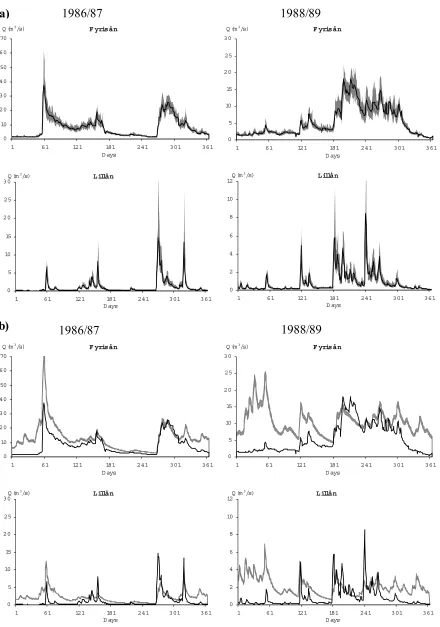
[image:10.595.73.514.66.689.2]F yrisån
0 10 20 30 40 50 60 70
1 61 121 181 241 301 361 D ays
Q (m3/s)
F yrisån
0 5 10 15 20 25 30
1 61 121 181 241 301 361 D ays
Q (m3/s)
Lillån
0 5 10 15 20 25 30
1 61 121 181 241 301 361 D ays
Q (m3/s) Lillån
0 2 4 6 8 10 12
1 61 121 181 241 301 361 D ays
Q (m3/s)
F yrisån
0 10 20 30 40 50 60 70
1 61 121 181 241 301 361 D ays
Q (m3/s)
F yrisån
0 5 10 15 20 25 30
1 61 121 181 241 301 361 D ays
Q (m3/s)
Lillån
0 5 10 15 20 25 30
1 61 121 181 241 301 361 D ays
Q (m3/s)
Lillån
0 2 4 6 8 10 12
1 61 121 181 241 301 361 D ays
Q (m3/s)
a)
b)
1986/87
1986/87
1988/89
1988/89
[image:11.595.87.527.66.693.2]Lillån
0 5 10 15 20 25 30
1 61 121 181 241 301 361
D ays Q (m3
/s)
F yriså n
0 10 20 30 40 50 60 70
1 61 121 181 241 301 361
D ays Q (m3
/s) F yriså n
0 5 10 15 20 25 30
1 61 121 181 241 301 361
D ays Q (m3
/s)
Lillån
0 2 4 6 8 10 12
1 61 121 181 241 301 361
D ays Q (m3
/s)
[image:12.595.60.528.72.390.2]1986/87
1988/89
Table 4. The Nash-Sutcliffe model efficiency (Reff) (1981-1990) for original streamflow and log-transformed streamflow.
GLUE LIKELIHOOD SIMPLELIKELIHOODMODEL FULLLIKELIHOODMODEL
Catchment Ecomag alone Ecomag alone Ecomag Ecomag alone Ecomag
+simple statistical model + full statistical model
Fyrisån 0.81 / 0.82 0.80 / 0.86 0.73 / 0.86 0.09 / -0.19 0.98 / 0.99 Sagån 0.57 / 0.65 0.61 / 0.71 0.61 / 0.66 0.29 / -0.29 0.94 / 0.97 Lillån 0.69 / 0.62 0.79 / 0.74 0.71 / 0.81 0.00 / -0.74 0.97 / 0.97
Örsundaån 0.75 / 0.75 0.65 / 0.71 0.63 / 0.77 0.26 / -0.28 0.95 / 0.97
Hågaån 0.63 / 0.67 0.65 / 0.70 0.63 / 0.77 0.24 / -0.30 0.96 / 0.98
Sävaån 0.77 / 0.79 0.65 / 0.72 0.63 / 0.78 0.17 / -0.26 0.95 / 0.97
Sävjaån 0.71 / 0.59 0.65 / 0.70 0.63 / 0.76 0.24 / -0.30 0.96 / 0.98
Stalbobäcken 0.57 / 0.54 0.65 / 0.71 0.63 / 0.77 0.27 / -0.26 0.97 / 0.98
Stabbybäcken 0.61 / 0.57 0.65 / 0.70 0.63 / 0.76 0.24 / -0.35 0.96 / 0.98
[image:12.595.44.540.498.704.2]Average 0.68 / 0.67 0.68 / 0.73 0.65 / 0.78 0.22 / -0.30 0.96 / 0.97
the statistical models together for only the two statistical likelihood models, are shown in Table 4.
Discussion
THE ILL-POSED PARAMETERS
The optimal Ecomag parameters are located in different parts of the parameter space for the two statistical likelihood models. This difference might explain why the Ecomag parameters are ill-posed for the simple likelihood model but well defined for the full likelihood model. The reason for the ill-posedness is probably that the hydrological model is non-linear. The properties of the Ecomag model may need investigation in more detail to find a smoother likelihood. The ill-posedness disturbs the estimation procedure. It leads, for instance, to having to decide whether the critical temperature for start of snow melt is 0.800 or 0.805oC, which
is trivial. A priori a smooth likelihood surface is desirbale; to achieve this it is possible to restrict the variances ω and τ to be much larger. These parameters will then lose their interpretation as the variance of the simulation errors. A second possibility is to define a function that smooths the likelihood surface. To find such a function, however, is not an objective in this paper and is open to further studies.
THE ROBUSTNESS OF THE LIKELIHOOD MODELS
The Reff values in Table 4 show that the streamflow estimates based on the simple likelihood model are as good as the estimates based on the GLUE likelihood for non-transformed streamflows, and better for the log-non-transformed streamflows. The Reff values indicate satisfactory or good simulation results for all catchments. Here, a minumum of 0.75 is classified as a good result and between 0.75 and 0.36 as satisfactory. The Reff values for the simple likelihood model fluctuate less between the catchments than the Reff values for the GLUE likelihood. The simple likelihood gives more robust streamflow simulations and is, therefore, the most suitable for simulation of streamflow in ungauged catchments. However, a cross-validation test is necessary to answer this question fully.
The fit to the observed record is almost perfect when Ecomag is combined with the full statistical model to simulate streamflow (Fig. 7a and Table 4). The auto-regressive term improves the streamflow estimation significantly. The Ecomag model alone, however, performs badly (Fig. 7b and Table 4)because the full likelihood (Eqn. 7) minimises not the simulation errors but rather the difference between the observed and simulated streamflow gradients. Moreover, the full likelihood behaves as a
black-box model on top of the Ecomag model. When the statistical and hydrological models are optimised simultaneously, one cannot be sure that the hydrological model alone gives the best possible estimates. The auto-regressive term of the likelihood might compensate for the mistakes of the Ecomag model. To obtain parameters that give better simulations for the hydrological model alone, there are two possible solutions within the Bayesian framework. The first is to define prior distribution for the Ecomag parameters that have small variances. The calibration procedure will then lose some freedom and the Ecomag model alone might give better simulations. The problem is, however, to have enough information to determine such well defined priors. The second solution is to formulate a penalised likelihood function for the Ecomag parameters, e.g. by requiring that the water balance for the hydrological model alone should be fulfilled to a certain degree.
ERRORS IN THE MODEL STRUCTURE AND TRANSFERABILITY OF SIMULATION ERRORS
The statistical parameters describe errors that arise from the model structure. The statistical parameters for the full likelihood model are not shown because it makes little sense to interpret them. The following comments relate to the estimated statistical parameters for the simple likelihood model shown in Fig. 4.
The variability between the catchment-dependent parameters µµµµµ and ωωωωω is larger than the variability between the process dependent parameters m and τττττ. This shows that the catchment properties are at least as important as the underlying hydrological processes for explaining the simulation errors of Ecomag.
directly in the parameterisation of the likelihood function. The simulation errors also depend on the underlying hydrological processes. This information is useful in a regional context and shows that it is possible to transfer knowledge about the simulation errors to ungauged catchments. The bias parameter (m) depends on the non-linear snow processes for temperatures between 2.5oC and
5.0oC and less on the water transport processes. Ecomag
over-estimates the streamflow when the temperature is above 5oC (m
1–m4), under-estimates when the temperature
is between –2.5oC and 5.0oC (m
5–m8), and over-estimates
slightly again for temperatures below –2.5oC relative to the
reference climate class (m13 = 0). The variance depends on the climate classes in a more complicated way. It is smallest for the reference climate class (τ13 = 0) and for temperatures
below –2.5oC (τ
9–τ11). For temperatures around 0oC, the
variance is highest when there is snow cover (τ6 and τ8).
For temperatures above 5oC, the variance is smallest when
there is snow cover and no precipitation (τ4). The variance
for rainfall-events (τΙ) has the same magnitude as that for precipitation and possible snow melt events when the temperature is around 0oC (τ
6). This implies that the
simulation of transport processes is as least as important as the simulation of snow processes for explaining the variance of the simulation errors.
ERRORS IN THE ECOMAG PARAMETERS
The estimated Ecomag parameter values and the width of the credibility intervals depend on the likelihood function (Fig. 5). The credibility intervals show that the estimated parameter uncertainty is much higher for the GLUE likelihood than for the two statistical likelihoods. The reason is that the GLUE likelihood punishes less than the statistical likelihoods for wrong simulations. The parameters estimated by the simple likelihood model are within the credibility intervals estimated by the GLUE likelihood, except for the vertical conductivity of horizon A and the conductivity of the groundwater zone. A reason for these two significant differences is that the GLUE likelihood operates on non-transformed streamflows, whereas the statistical likelihood operates on log-transform streamflows. The GLUE likelihood therefore puts more weight on high streamflow values in the parameter estimation. The Ecomag parameters estimated by the full likelihood model differ significantly from the GLUE estimates for five parameters; among them the evaporation, the horizontal conductivity of horizon A and the thickness of horizon A are the most different. These three parameters might be the most important to control to obtain better results for the full likelihood model.
CREDIBILITY INTERVALS FOR SIMULATED STREAMFLOW
The credibility intervals for the simulated streamflows calculated from the simple model indicate that the uncertainty in the Ecomag parameters (Fig. 5b) is less important than the errors in the model structure (Figs. 5a, 6a) model for explaining the total modelling uncertainty.
The statement above depends on how the parameter and model uncertainty is represented. The use of a statistical model for the simulation errors to represent the uncertainties in the model structure has some drawbacks, particularly because it does not include the physics of the hydrological system, e.g. the water balance and the process dynamics. If some flood peaks are estimated one day too early or too late, the estimated variance in the statistical model might become relatively high. Such mistakes are serious in the discharge domain but not in the time domain. The credibility intervals in Fig. 5a indicate a high uncertainty in the hydrological model, and a modeller seeks more confidence in a model than these credibility intervals indicate. Instead of constructing a statistical model for the simulation errors, the GLUE and the multi-objective method utilise the flexibility in the model parameters to describe the total modelling uncertainty. In the GLUE framework it is possible to require that the parameter uncertainty should be high enough to let a 95% credibility interval for the streamflow cover 95% of the observed streamflows. In any event, the credibility intervals for the simulated streamflow based on a GLUE likelihood (Fig. 7) are much wider than those based on a statistical likelihood (Fig. 5b). This way of representing the uncertainty utilises knowledge of the dynamics of the hydrological system that is implemented in the model. It is not necessary to invent a new model to describe the uncertainties. A serious disadvantage for this uncertainty estimation is that the model structure might not be flexible enough to describe all the uncertainties in the simulations. This is clearly seen in Fig. 7 where the observed values far exceed the estimated credibility intervals for a short period in 1988/89.
Conclusions
A full Bayesian formulation has been applied to estimate regional parameters for the Ecomag model adapted to the NOPEX area. The hydrological parameters and the statistical parameters for the simulation errors are estimated simultaneously. Two statistical likelihood functions and one GLUE likelihood function have been used to see how different formulations influence the results.
reasonable precision and robust model parameters are obtained. A simple statistical likelihood model gives more robust parameter estimates than a GLUE-likelihood and is, therefore, preferred for regionalisation of the hydrological parameters. In this paper, the parameters in the Ecomag model have been regionalised. If the simulation errors of an ungauged catchment in the same area are of interest, the statistical parameters have to be regionalised as well. The results show that the simulation errors depend on the climate so that some knowledge of the simulation errors can be transposed to ungauged basins. The simulation errors also depend on the catchments; hence, catchment characteristics can be used to transfer more knowledge about the simulation errors to ungauged catchments. The variance of the simulation errors will be under-estimated for some catchments and over-estimated for others as a result of the regionalisation.
The model uncertainty is more important than the parameter uncertainty in explaining the errors in the simulated streamflow. However, this conclusion assumes that a statistical model for the simulation errors is used as the likelihood function. In hydrology, alternative formulations such as GLUE and the multi-objective method are used to estimate the modelling uncertainties. These two methods utilise the flexibility in the model parameters to estimate the uncertainty, and the present results show that the parameter uncertainty is larger in the GLUE than in the Bayesian framework.
Further studies might go in two directions. The first is to investigate how to represent and parameterise the modelling uncertainties and to compare the Bayesian method with both the multi-objective and the GLUE methods. It would also be interesting to investigate Bayesian methodology further. Important tasks are to find a penalised likelihood function for the AR(1) likelihood, include spatial correlations in the likelihood model, and to include the uncertainty in the precipitation and streamflow observations in the total modelling uncertainty which will not necessarily increase much because the four error sources might interact and cancel each other out. The second direction is to use the tools presented here to develop and, hopefully, improve the parameterisation of the hydrological processes. It is possible to compare different process formulations and choose the the most suitable for regional applications. Then, it might be important to include multiple responses in the model evaluation, e.g. soil moisture, ground water and snow cover.
References
Abdulla, F.A. and Lettenmaier, D.P., 1997. Application of regional parameter estimation schemes to simulate the water balance of a large continental river. J. Hydrol., 197, 258–285.
Beven, K.J. and Binley, A.M., 1992. The future of distributed models - model calibration and uncertainty prediction. Hydrol. Process., 6, 279–298.
Boyle, D.P., Gupta, H.V. and Sorooshian, S., 2000. Towards improved calibration of hydrologic models: Combining the strengths of manual and automatic methods. Water Resour.Res., 36, 3663–3674.
Chib, S. and Greenberg, E., 1995. Understanding the Metropolis-Hastings algorithm. Amer. Statist., 49, 327–335.
Engeland, K., 2002. Parameter estimation in regional hydrological models. PhD dissertation, Faculty of Mathematics and Natural Sciences, University of Oslo, Norway, 157 pp.
Engeland, K., Gottschalk, L. and Tallaksen, L., 2001. Estimation of regional parameters in a macro scale hydrological model.
Nord. Hydrol., 32, 161–180.
Gupta, H.V., Sorooshian, S. and Yapo, P.O., 1998. Towards improved calibration of hydrologic models: Multiple and noncommensurable measures of information. Water Resour. Res., 34, 751–763.
Halldin, S., Gottschalk, L., van de Girend, A.A., Gryning, S.E., Heikinheimo, M., Högstrom, U., Jochum, A. and Lundin, L.C., 1995. Science plan for NOPEX, NOPEX Technical report No. 12, Institute of Earth Sciences, Uppsala University, Sweden, 38 pp.
Halldin, S., Gryning, S.E., Gottschalk, L., Jochum, A., Lundin, L.C. and Van de Griend, A.A., 1999. Energy, water and carbon exchange in a boreal forest landscape – NOPEX experiences.
Agr. Forest Meteorol., 98-99, 5–29.
Hastings, W.K., 1970. Monte Carlo sampling methods using Markov chains and their applications. Biometrika, 57, 97–109. Klemeš, V., 1986. Operational testing of hydrological simulation
models. Hydrolog. Sci. J., 31, 13–24.
Krzysztofowicz, R., 1999. Bayesian theory of probabilistic forecasting via deterministic hydrologic model. Water Resour. Res., 35, 2739–2750.
Kuczera, G., 1983. Improved parameter inference in catchment models 1. Evaluating parameter uncertainty. Water Resour. Res., 19, 1151–1162.
Langsrud, Ø., Frigessi, A. and Høst, G., 1998. Pure model error
of the HBV-model, Hydra Note 4/1998, Norwegian Water
Resources and Energy Directorate, Oslo, Norway, 28 pp. Lundin, L.C., Halldin, S., Nord, T. and Etzelmüller, B., 1999.
System of information in NOPEX – retrieval, use, and query of climate data. Agr. Forest Meteorol., 98-99, 31–51.
Motovilov, Y.G., Gottschalk, L., Engeland, K. and Rodhe, A., 1999. Validation of a distributed model against spatial observations. Agr. Forest Meteorol., 98-99, 257–277. Nash, J.E. and Sutcliffe, J.V., 1970. River flow forecasting through
conceptual models Part 1 - A discussion of principles. J. Hydrol., 10, 282–290.
Refsgaard, J.C., Rosbjerg, D. and Markussen, L.M., 1983. Application of Kalman filter to real-time operation and to uncertainty analyses in hydrological modelling. In: Scientific procedures applied to the planning, design and management of
water resource systems, E. Plate and N. Buras (Eds.),
(Proceedings of the Hamburg symposium), IAHS Publication
147, 273–282.
Refsgaard, J.C. and Knudsen, J., 1996. Operational validation and intercomparison of different types of hydrological models.,
Water Resour.Res., 32, 2189–2202.
Romanowicz, R., Beven, K.J. and Tawn, J.A., 1994. Evaluation of predictive uncertainty in nonlinear hydrological models using a Bayesian approach, In: Statistics for the environment 2: Water related issues, V. Barnett and K.F.Turkman, (Eds.) Wiley, Chichester, UK, 297–317.
Seibert, P., 1994. Hydrological characteristics of the NOPEX research area. Nopex Technical Report No. 3, Institute of Earth Sciences, Uppsala University, Sweden. 51 pp.
Sorooshian, S., 1991. Parameter estimation, model identification, and model validation: conceptual-type models. In: Recent Advances in the Modelling of Hydrologic Systems, D.S. Bowles and P.E. O’Connell (Eds.) NATO ASI Series, 345, 443–467. Storm, B., Jensen, K.H. and Refsgaard, J.C., 1988. Estimation of
catchment rainfall uncertainty and its influence on runoff prediction. Nord.Hydrol., 19, 77–88.
Thorsen, M., Refsgaard, J.C., Hansen, S., Pebesma, E., Jensen, J.B. and Kleeschulte, S., 2001. Assessment of uncertainty in simulation of nitrate leaching to aquifers at catchment scale. J. Hydrol., 242, 210–227.
Appendix
The vector of all parameters is Z and π their posterior densities, q their proposal densities, m the number of iterations, ns the number of statistical parameters, and ne the number of hydrological parameters. The statistical parameters are located in Z1–Zns and the hydrological parameters are located in Zns+1–Zns+ne. The algorithm involves the following steps:
z for L = 1,2 ,...m, let Z(L) be the current state of the chain. z draw I randomly from 1,2 ,...ns+1 (each only once for
each iteration) z if I = ns+1 ( )L
n n
ns s e
Z
x= +1: + else x=ZI( )L
z draw a new value for x* from a specified irreducible proposal distribution qI:
( )
**~q x,x
x I where x x( ) j I
L j
j= ∀ ≠
* (A1)
z compute the acceptance probability
( )
( )
( )
[ ]
[ ]
= * * * * , , , 1 min , x x q x x x q x x x a I I π π (A2)z If I = ns+1 then
( )
( )
( )
− = + + + * * * 1 : 1 , 1 y probabilit with , y probabilit with x x a x x x a x ZL n n ns s eelse ( )
( )
( )
− = + * * * 1 , 1 y probabilit with , y probabilit with x x a x x x a x ZL I (A3)
As the ratio of two posterior densities is calculated, this algorithm does not require the normalisation constant of the posterior probability density (Eqn. 2).
THE PROPOSAL DENSITIES
The proposal densities (Eqn. A1) must be decided. A random walk algorithm is used, i.e. the proposal density depends on the current state of the chain. For all parameters, uniform proposal densities centred at the current parameter value are defined. No values outside the uniform prior distributions are proposed, because then the acceptance probability is zero. The amplitudes of the uniform priors are kept constant to simplify the acceptance probability.
THE ACCEPTANCE PROBABILITIES
For the µµµµµ, m, ωωωωω, τττττ and the Ecomag parameters, the uniform proposal densities are constructed to have a constant variance. As a result q
(
x,x*) (
qx*,x)
= , and the acceptance
probability (Eqn. A2) can be simplified to the ratio of the new and old posterior densities:
(
)
( )
( )
= x x x x a π π * * min 1,, (A10)
For the ααααα and βββββ parameters it is necessary to use Eqn. (A2) to calculate the acceptance probabilities.
INITIALISATION OF THE MH ALGORITHM
The initial values of the parameters might in principle be chosen randomly within the prior distribution. The MH-algorithm will then converge towards the area of highest probability. This convergence is rather slow. To save computing time, the parameters are optimised with respect to the likelihood function, and the optimised parameters are used as initial values for the MH algorithm.
TUNING THE MH ALGORITHM