www.hydrol-earth-syst-sci.net/14/1537/2010/ doi:10.5194/hess-14-1537-2010
© Author(s) 2010. CC Attribution 3.0 License.
Earth System
Sciences
Integrated response and transit time distributions of watersheds by
combining hydrograph separation and long-term transit time
modeling
M. C. Roa-Garc´ıa1,3and M. Weiler2
1Land and Food Systems, University of British Columbia, 2357 Main Mall, Vancouver, B.C., V6T 1Z4 Canada 2Institute of Hydrology, University of Freiburg, Fahnenbergplatz, 79098 Freiburg, Germany
3Fundaci´on Evaristo Garc´ıa, A.A. 4443, Cali, Colombia
Received: 6 December 2009 – Published in Hydrol. Earth Syst. Sci. Discuss.: 6 January 2010 Revised: 25 May 2010 – Accepted: 18 July 2010 – Published: 13 August 2010
Abstract. We present a new modeling approach
analyz-ing and predictanalyz-ing the Transit Time Distribution (TTD) and the Response Time Distribution (RTD) from hourly to an-nual time scales as two distinct hydrological processes. The model integrates Isotope Hydrograph Separation (IHS) and the Instantaneous Unit Hydrograph (IUH) approach as a tool to provide a more realistic description of transit and response time of water in catchments. Individual event simulations and parameterizations were combined with long-term base-flow simulation and parameterizations; this provides a com-prehensive picture of the catchment response for a long time span for the hydraulic and isotopic processes. The proposed method was tested in three Andean headwater catchments to compare the effects of land use on hydrological response and solute transport. Results show that the characteristics of events and antecedent conditions have a significant influ-ence on TTD and RTD, but in general the RTD of the grass-land dominated catchment is concentrated in the shorter time spans and has a higher cumulative TTD, while the forest dominated catchment has a relatively higher response dis-tribution and lower cumulative TTD. The catchment where wetlands concentrate shows a flashier response, but wetlands also appear to prolong transit time.
Correspondence to: M. C. Roa-Garc´ıa ([email protected])
1 Introduction
Water management with the aim to sustain catchment eco-logical services requires an understanding of the hydrologic cycle. Comparative analysis of catchment behavior allows observing the effects of human activities on the amount and rate of water flows, the effects of land use change on wa-ter quantity and quality, the persistence of soluble contami-nants in catchments, and the vulnerability of ecosystems to be impacted by climate change. Comparing flows, residence time and transit time of water from catchments with simi-lar size, topography and soil type, enables us to understand the influence that particular catchment components and pro-cesses have on catchment response to precipitation and to dry periods.
Stable water isotopes have been used in hydrology for two purposes: (1) to identify the temporal variations of water sources for baseflow and for individual storms; and (2) to identify the source of runoff during an event, e.g. whether it comes from rain or snowmelt (event water) or from water stored in the watershed prior to the event (groundwater, soil water, lakes etc.) (Vitvar et al., 2005). This knowledge has been used to understand the interactions between precipita-tion, runoff pathways and runoff generation processes, and as a proxy for the capacity of a catchment to store water and chemicals and regulate its flow (Soulsby et al., 2009).
of drainage basins (Sherman, 1932; Clark, 1945; Barnes, 1940; Hewlett and Hibbert, 1967). Later, tracers have been used in a more objective way to separate the storm hydro-graph. Stable isotope hydrograph separations (IHS) (Pin-der and Jones, 1969; Sklash et al., 1976) and conservative geo-chemical tracing (Hooper and Shoemaker, 1986) have been developed into common tools in watershed hydrology (Kendall and McDonnell, 1998). These tracer-based sep-aration approaches have the advantage of providing more process-based information about temporal and geographic sources of runoff.
Lumped transport models to estimate the transit time of water in catchments or other hydrological systems (ground-water, unsaturated zone) have been developed in parallel to predict the transit time distribution (TTD) and mean transit time (MTT) of a system (Maloszewski and Zuber, 1982). These models have been used mostly under baseflow con-ditions in catchments since an important assumption is sta-tionarity of runoff. A detailed review of the different models, applications and assumptions can be found in McGuire and McDonnell (2006).
Other approaches to simulate and analyze TTD include one developed by Kirchner et al. (2001), which combined different transport models (advection-dispersion, exponen-tial and gamma models) and the observed fractal scaling in rainfall and catchment runoff and chemistry in the spectral domain. This approach implies a large number of parameters that are not possible to test in models that are not disaggre-gated into individually parameterized compartments (Kirch-ner et al., 2001). Botter et al. (2005) discussed stochastic models that embed spatial variability and uncertainty into a mathematical framework of a reduced number of param-eters. They evaluated models including the mass response functions which they suggest as an appropriate generic trans-port model for catchments. More recently Botter et al. (2010) have explored non-linearities in travel time distributions as-sociated with time-varying rainfall, runoff and evapotranspi-ration processes, proposing a transport model that considers catchments as nonlinear systems with memory.
Despite the common use of IHS and transit time mod-eling in hydrology, the combination and integration of the two approaches has not yet been explored. Our approach builds upon the work of McDonnell et al. (1999) and Weiler et al. (1999), whereby the temporal variability in rainfall iso-topic composition during an rainfall event is used to model event based transit time distribution (analogous to the annual time series approach of Maloszewski and Zuber, 1982) and to compute event and pre-event water contributions to storm runoff. We thus estimate event water transit time distribu-tions for discrete events (building upon Unnikrishna et al., 1995). In effect, their work was an attempt to combine the process merits of tracer-based hydrograph separation with the hydraulic transfer function approach of the unit hydro-graph in an effort to increase the information gained from the storm hydrograph. The new method of hydrograph
sepa-ration proposed in this paper embraces the temporal variabil-ity of rainfall isotopic composition, but includes a new trans-fer function for event water and pre-event water determined from the time-variable event water fraction. A transfer func-tion representing the runoff response (i.e. the instantaneous unit hydrograph) is used to constrain the event residence time distribution and the hydrograph components. This trans-fer function approach overcomes many of the limitations of traditional two-component hydrograph separations (Buttle, 1994) and provides separate representations of runoff and tracer responses to storm events that are used to improve de description of hydrologic processes. We argue in this paper that both responses are essential to understand catchment be-havior, since one response (i.e. the transit time) represents ac-tual conservative solute travel time (i.e. along flowpaths) and the other represents hydraulic dynamics (e.g. rainfall-runoff response).
We present a new methodology that combines the isotope hydrograph separation and long term transit time modeling to provide realistic information about the response and tran-sit time of water in catchments over several orders of tempo-ral scales. We use this model to compare the effect of land use on the hydrological response of three small headwater catchments in the mountains of Colombia, that constitute the water source for a municipality of 15 000 people.
2 Methods
2.1 Study site and dataset
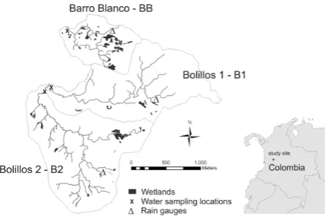
Fig. 1. Location of study site and the three small headwater catch-ments compared. The detailed map shows he wetlands found in each of the three catchments.
and imogolite, which combined produce soils of high water holding capacity.
The catchments (B1, B2 and BB) differ in size and land use (Table 1). BB is the smallest catchment, but has the largest proportion of wetlands. B2 is the largest catchment with the highest proportion of grasslands. And B1 is smaller than B2 but has a larger proportion of natural and riparian forest.
Streamflow was monitored at the outlet of the three catch-ments. Water level was recorded every 15 min from June 2005 until May 2007 with three AquiStar PT2X Smart Sen-sors© at the catchment outlet. The water level data se-ries were converted into discharge measurements with stage-discharge relations using 62, 44 and 50 stage-discharge measure-ments for catchmeasure-ments B1, B2 and BB, respectively. A nat-ural cross-section was used in each of the streams to do the flow measurements with an OTT flow meter. Stage/Q dis-charge relationships were obtained as equations of the form
Q=k(h–ho)a using solver in excel (details of these
equa-tions can be found in Roa-Garc´ıa, 2009). Average annual discharge during the period of monitoring was 2400 mm for B1, 2490 mm for B2 and 2047 mm for BB. Precipitation was measured using three Hobo Pro data logging rain gauges lo-cated in each catchment and precipitation for the thee catch-ments was 3264 mm for B1, 3020 mm for B2 and 3141 mm for BB. All rain gauges were located on grassland sites at between 2100 and 2135 m of elevation.
Rain samples were taken every two weeks from November 2005 until May 2007 (n=39). Rain was collected according to guidelines from the isotope hydrology laboratory of the International Atomic Energy Agency – IAEA (IAEA, 2002), to prevent fractionation through temperature variations or di-rect exchange of rain water with the atmosphere. The water accumulated every two weeks was mixed in the container and a sample was taken at the end of the sampling period. At all
stream gauging stations, stream water samples were manu-ally taken every two weeks, from May 2006 to May 2007 (n=74).
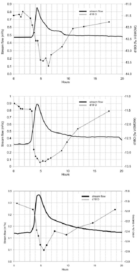
An event is defined as precipitation equal or larger than 2 mm that ends when there has been no precipitation for the following 2 h. Seven storm events were sampled during two rainy seasons in 2006 and 2007, of which five events were se-lected for modeling due to their completeness: 14 November of 2006 (event 2), 21 November 2006 (event 3), 7 April 2007 (event 5), 18 April 2007 (event 6) and 25 April 2007 (event 7). The rain samples were taken manually and a group of six people participated in the collection of samples for each event. The sequence of rain samples was determined by the speed at which vials could be filled with rain. From the three streams an initial sample was taken before the rain started. Once the water level started rising, samples were taken ev-ery 20 min until the peak was reached when another sample was taken. After the peak, four samples were taken every 30 min and then every two hours until the water level re-turned to the same water level in the stream previous to the beginning of the storm event. The number of samples was 104 for event 2, 83 for event 3, 71 for event 5, 95 for event 6, and 86 for event 7. Precipitation and discharge samples were taken in high density polyethylene scintillation vials with cone caps. The oxygen isotopic composition of sam-ples was determined with a Finnigan Delta XP IRMS and the GasBench II using the classical headspace-equilibration technique. Theδ18O values are reported in per mil (‰) rel-ative to the standard (VSMOW) with an analytical error of ±0.08‰. Figure 2 shows the isotope signal for each of the three streams for event 2, showing similarities of isotope sig-nal response for the three streams. Figure 3 shows the com-parison between precipitation amount and isotopic composi-tion for the present study. For the long term analysis, the iso-topic composition data of precipitation was paired with the long term precipitation data of the closest Global Network of Isotopes in Precipitation (GNIP) stations (Pereira and Bo-gota). The correlations of the monthly average of precipi-tation for the period 1971–2007 of this climate sprecipi-tation with the precipitation of the present study for the years 2005 and 2006 was of 0.9 and 0.8 and the correlation of the overlap-ping monthly isotope18O values werer2=0.77.
2.2 Estimating RTD and TTD for events and
baseflow conditions
Fig. 2. Stream discharge and stream isotope signal for event 2 for B1 (top), B2 (center) and BB (bottom).
the catchment and the time they are observed in the catch-ment outlet (Vitvar et al., 2005). Mean Response Time (MRT) on the other hand, is an indicator of the rainfall-runoff response as it represents the speed and volume of outflow with which a catchment responds to water input (precipita-tion). Since the fluctuations in hydraulic head (the driving force in water flux) can propagate much faster than individ-ual water molecules, the MRT is expected to be shorter than the MTT. The TTD describes the distribution of times that each molecule of water takes to arrive at the catchment out-let from all locations in the catchment (McGuire and
Mc-Table 1. Proportion of land use for each catchment.
B1 B2 BB
Areas ha % ha % ha %
Riparian and natural forest 81 51 49 27 15 25
Plantation forest 28 17 2 1 3 5
Grasslands 48 30 124 69 39 62
Wetlands 1 1 3 1 4 6
Roads and buildings 1 1 2 1 1 1
Total area 159 100 180 100 62 100
Donnell, 2006). The response time distribution or RTD is the integrated response time of a catchment to a unit rainfall input and is similar to the unit hydrograph concept.
The models to estimate RTD and TTD for individual events and under baseflow condition were further developed from the TRANSEP model, which is a quantitative approach to describe the transit time and transmittance of hydraulic be-havior to help understand the relationship between pre-event and event water delivery to streams (Weiler et al., 2003). It uses water flux and isotopic data from precipitation and streamflow to derive transfer functions of runoff, event and pre-event water by capitalizing on the temporal variation of rainfall tracer composition. The transfer function can be chosen from transfer functions previously defined including the exponential distribution, the exponential piston-flow dis-tribution and the advection-dispersion model (Maloszewski and Zuber, 1982), the gamma distribution (Kirchner et al., 2001), or the two parallel linear reservoirs model (Weiler et al., 2003). Weiler et al. (2003) tested these models and obtained best results from the two parallel linear reservoirs (TPLR). Other studies (Hrachowitz et al., 2009; McGuire et al., 2005) also showed that the TPLR model produces good results. The TPLR was the transfer distribution used for the present study.
[image:4.595.311.544.87.183.2]Fig. 3. Isotopic signal in precipitation and streams compared with the amount of precipitation for 2-week periods.
and McDonnell, 2006). Therefore, the input data was ex-tended by correlating the observed isotopic data to the near-est long-term climate station (Bremen, CRQ) and extending the input time series to five years.
The models to estimate RTD for the short and long time scale are both simple runoff models that simulate stream-flow by a non-linear and a linear module, similar to a variety of instantaneous unit hydrograph (IUH) based models (Bras, 1990). The non-linear module is the loss function generat-ing an effective precipitation time series (Jakeman and Horn-berger, 1993):
s(t )=b1p(t )+
1−b−21s(t−1t ) (1)
peff(t )=p(t )s(t ) (2)
wherepeff(t ) is the effective precipitation, s(t ) is the
an-tecedent precipitation index that is calculated by exponen-tially weighting the precipitation backward in time accord-ing to the parameterb2. The parameterb1 scales the total
simulated runoff over the simulation period (similar to a run-off coefficient) and thus can be determined directly from the rainfall- runoff data. The runoff coefficient rc for each tem-poral scale can be defined as the total effective precipitation divided by the total precipitation. The runoff coefficients for
the events are a reflection of runoff generation processes and storage; for the longer time scale, the difference between pre-cipitation and effective prepre-cipitation is due to evapotranspi-ration. The linear module describes a convolution of the ef-fective precipitation and runoff transfer function:
Q(t )= Z t
0
g(τ ) peff(t−τ ) dτ (3)
where g(τ )is the response time distribution (RTD), defined for the long term (b)and event (e)scale, and thus the rainfall-induced response of catchment runoff.
To estimate the streamflow concentration C(t ) for the baseflow model we use the tracer mass flux instead of the tracer concentration since the tracer signal depends on the ac-tual tracer mass flux, which depends on the effective precip-itation (Stewart and McDonnell, 1991; Weiler et al., 1999):
C(t )= Rt
0Cin(t−τ ) peff(t−τ ) hb(τ ) dτ
Rt
0peff(t−τ ) hb(τ ) dτ
(4) wherehb(τ )is the long-term transit time distribution andCin
is the observed input concentration in the precipitation. As introduced into the TRANSEP model, the event water tran-sit time distributionhe(τ )can be calculated in a similar way
event and pre-event water runoff during the events. The con-centrationC(t )in the stream is then given by (Weiler et al., 2003):
C(t )= Rt
0Cin(t−τ ) peff(t−τ ) f (t−τ ) he(τ ) dτ
Rt
0peff(t−τ ) f (t−τ ) he(τ ) dτ
(5) The main difference to Eq. (4) isf , the fraction of effec-tive precipitation that becomes event water (i.e. “new” wa-ter), andhe(τ )is the transfer function of the event water (i.e.
the transit time distribution). The denominator of Eq. (5) is equal to the event water runoff (Weiler et al., 2003) and the total event water fractionF can then be derived. The units of nominator and denominator of Eq. (5) are (Volume/Time) to calculate the event water fraction.
As already discussed we use the two parallel linear reser-voirs as our transfer function for the RTD and TTD and for both time scales:
g(τ )=hb(τ )=he(τ )= φ τf exp −τ τf + 1−φ
τs exp −τ τs (6) Whereτf andτs are the mean response or transit times of
the fast and slow responding reservoirs, respectively. The parameterφ defines the partition of the input into the fast responding reservoir.
We used ant colony optimization to the inverse estimation problem of the unknown parameters (Abbaspour et al., 2001) for both time scales. It has been shown that this technique efficiently finds the optimum solution for a wide range of applications. First, the parameter of the response time model was optimized using precipitation as input and streamflow as output. Second, the parameters of the transfer time model were optimized adding the observed isotope concentration for precipitation and streamflow. This stepwise optimization technique ensures that the inverse problem is not ill posed and that the parameters are identifiable (Weiler et al., 2003).
2.3 Combining RTD and TTD from events and
baseflow modeling
The estimated RTD and TTD for the two time scales (min-utes for the events and days for the baseflow) are describing a hydrological system (i.e. watershed) with different tempo-ral resolution. In order to derive a RTD or TTD distribution that describes a catchment from minutes to years, we can combine the two distributions for the events and the base-flow. To do this, we select the distribution from an individual event and combine it with the overall distribution from the baseflow analysis. This can be done for different events and the RTD or TTD will show the time variant behavior of the catchment according to the event characteristics. This is sim-ilar to the observations made by McGuire et al. (2007). The combined RTD (gτ )and TTD h(τ )is then given by:
g(τ )=rcege(τ )+(1−rce)gb(τ ) (7)
h(τ )=[rceF he(τ )+(1−rceF )hb(τ )]rcb (8)
The integral of the RTD will be unity, but as can be seen in Eq. (8), the integral of the TTD can be less than unity. The idea behind this new concept is that for an open system like a catchment, part of the water molecules entering the sys-tem as precipitation will leave the catchment not through the stream but by evapotranspiration. Hence, a TTD can in a strict way not approach unity for most catchments as part of the water molecules that entered the system during a precipi-tation event never reach the stream. This idea is similar to the stochastic concept of an evapotranspiration time probability distribution function pdf proposed by Botter et al. (2010).
3 Results
3.1 RTD and TTD of rainfall-runoff events
Five sampled storms were analyzed using TRANSEP for the three catchments. The results are shown in Table 2. Re-sults include event water, defined as the proportion of stream discharge during an event that originates from precipitation (Buttle, 1994) and runoff coefficient which corresponds to the proportion of rainfall that becomes stream discharge dur-ing an event. For each of the two processes (transit of indi-vidual water molecules and the response of catchments) three parameters are optimized: the transit/response time of the fast reservoir (τf), the transit/response time of the slow
reser-voir (τs)and the portion of the total discharge corresponding
to the fast reservoir (8)for individual events.
The model was generally able to predict the observed runoff response as the Nash-Suttcliff Efficiency is larger than 0.8 for almost all events. As shown in Table 2, efficiency val-ues of the simulation indicate that the prediction of the iso-topes variation in the streamflow with TRANSEP was also acceptable. Generally, the RTD is dominated by the fast reservoir with a very rapid response time below 1 h. The TTD is prolonged over a longer period, but dominated by the fast reservoir. For a couple of events, the two linear reser-voirs are simplified to an exponential model since the por-tion of the total discharge corresponding to the fast reservoir is equal to unity.
Table 2. Parameters of response and transit time model applied to individual events.
total Antecedent TTD RTD
rain in precipitation Max
N-event (mm) I15 Event Measured Simulated Q C isotope
Event Catchment (mm) 1 day 3 days (mm) water RC RC Efficiency Efficiency τf(h) τs(h) 8(-) τf(h) τs(h) 8(-) Samples
2 B1 24 18 88 5 23% 10% 10% 0.95 0.68 2.2 82 0.70 0.1 1.6 0.65 18
6 B1 38 2 5 10 24% 11% 10% 0.85 0.63 1.5 120 1.00 0.1 2.2 0.73 19
7 B1 30 14 30 14 32% 5% 5% 0.54 0.86 1.5 82 0.70 0.1 2.1 0.40 11
2 B2 24 16 66 3 25% 21% 20% 0.90 0.78 4.7 120 0.60 0.1 1.1 0.47 18
5 B2 24 1 3 6 40% 14% 13% 0.80 0.86 2.3 40 0.88 0.1 2.1 0.62 19
6 B2 31 2 5 11 21% 28% 27% 0.98 0.48 0.6 95 0.30 0.1 0.6 0.47 16
2 BB 16 35 95 4 12% 25% 25% 0.96 0.48 3.3 120 1.00 0.1 2.4 0.78 13
3 BB 21 7 29 9 27% 36% 36% 0.95 0.88 1.8 120 0.97 0.1 2.3 0.80 15
5 BB 16 1 6 7 14% 19% 19% 0.76 0.59 2.7 120 0.90 0.1 1.8 0.69 15
RC = runoff coefficient
Efficiency = Nash-Sutcliffe Efficiency (unitless with a maximum of (1) providing a goodness-of-fit measure between observed and simulated discharge (Q) and isotope concentrations (C)
τf(h) = Transit or response time of fast reservoir
τs(h) = Transit or response time of slow reservoir 8(-) = Portion of fast reservoir
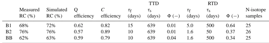
Table 3. Parameters of response and transit time model applied to baseflow.
TTD RTD
Measured Simulated Q C τf τs τf τs N-isotope
RC (%) RC (%) efficiency efficiency (days) (days) 8(−) (days) (days) 8(−) samples
B1 68% 72% 0.62 0.82 15 639 0.01 5.0 500 0.64 25
B2 76% 76% 0.57 0.89 10 639 0.01 1.6 50 0.37 26
BB 62% 63% 0.59 0.79 10 639 0.04 1.6 500 0.34 25
RC = runoff coefficient
Efficiency = Nash-Sutcliffe Efficiency (unitless with a maximum of 1) providing a goodness-of-fit measure between observed andsimulated discharge (Q) and isotope concentrations (C)
τf(h) = Transit or response time of fast reservoir
τs(h) = Transit or response time of slow reservoir 8(−) = Portion of fast reservoir
Antecedent precipitation combined with the size of the event, are major factors in determining the percentage of event water in the total discharge. Event 2 happened dur-ing relative wet antecedent conditions (66–95 mm within 3 days) producing relatively small event water contributions in all catchments, particularly in BB with the wettest antecedent conditions. All other events are characterized by drier an-tecedent conditions and generate, in general, more event wa-ter combined with a smaller runoff coefficient. Analysis of more events would have been necessary to provide a more consistent picture among the factors influencing runoff gen-eration and event water contribution.
3.2 RTD and TTD of baseflow
Results of the Transit Time model for the baseflow samples taken every two weeks are shown in Table 3. The three catch-ments have relatively high yields. Runoff coefficient – RC is defined as the proportion of rainfall that becomes stream discharge on an annual basis. B2, with a RC of 76% is the catchment with the smallest infiltration and storage
capac-ity when it rains, and thus a larger proportion of rainfall be-comes runoff. BB, despite having a similar percentage of for-est cover than B2, has the lowfor-est RC, pointing to the higher proportion of wetland area that would contribute to store wa-ter and preventing a higher proportion of runoff.
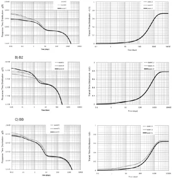
[image:7.595.59.529.316.392.2]Fig. 4. Response Time Distribution – RTD for the three catchments for event 2: probability density function – pdf (left), cumulative density function – cdf (right).
Fig. 5. Transit Time Distribution – TTD for the three catchments for event 2: probability density function – pdf (left), cumulative density function – cdf (right).
response time for B2. Catchment B2, despite a relatively large slow reservoir portion, has a short MRT due to its short MRT for the slow reservoir.
3.3 Comparing integrated RTD and TTD
The integration of event and baseflow data to generate RTD and TTD allows a comparison of catchments on a long time scale by incorporating the influence of individual events. Figure 4 compares the response of the three studied ments for event 2, which was a relatively large event in catch-ments B1 and B2 where 1-day antecedent precipitation was low and a medium size event for catchment BB (Table 2) where 1-day antecedent precipitation was higher. The result-ing RTD curves which illustrate the hydrological response of the catchments show a significantly shorter RTD for catch-ment B2. This is influenced by the land use differences be-tween the three catchments, since B2 is the catchment domi-nated by grasslands with a more limited water storage capac-ity than the catchments dominated by forest or with a signif-icant portion of wetlands. Additionally the curves show the effect that antecedent precipitation conditions have on RTD at the short time scale. These curves also show that B1, the forest dominated catchment, had the slowest response and hence the largest overall storage.
Differences between the TTD of the three catchments can be seen in the probability and cumulative distribution func-tion of the TTD as shown in Fig. 5. The large differences ob-served between the three catchments for the short times are determined by the runoff coefficients of the different events, which in turn respond to the influence of the size and inten-sity of the event and the antecedent precipitation conditions in each of the catchments. The cumulative TTD in the longer time scale show the influence of vegetation on the total evap-otranspiration flux which in turn influences the total amount of water that leaves the catchment by streamflow. The three curves show that the catchment with the highest percentage of wetlands (BB) is the catchment that looses more water in the longer time range through evapotranspiration, followed by the catchment dominated by forests (B1). Also the catch-ment with the highest proportion of wetlands (BB) has the highest proportion of water leaving the watershed within the first day.
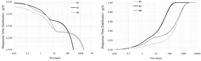
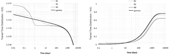
Fig. 6. Probability density function – pdf of Response Time Distribution (RTD –g(T )) and cumulative probability density function – pdf of Transit Time Distribution (TTD –h(T )) in the left and right columns, respectively.
other two catchments that show a higher frequency of longer response suggesting the influence of forests and wetlands as a long term water storage.
The comparison of the cumulative TTD for the individual catchments in the right column of Fig. 6 shows a similar pic-ture as for the RTD, but the variability of cumulative event water contribution among rainfall events is much smaller than the variability of runoff response and runoff coefficients among events. In the right column of Fig. 6 it is shown that the proportion of water leaving the watershed within the first 10 days is very similar for most events and below 10% for all watersheds, but smaller for B1. It is also apparent that BB looses more water to evapotranspiration, as the cumulative TTD in the longer time scale is smaller than for the other two catchments.
4 Discussion
4.1 A new response time and transit time distribution
Fig. 7. Transit Time Distribution – TTD for the three catchments for event 2 as shown in Fig. 3 but including a fitted gamma distribution (black line): probability density function – pdf (left) and cumulative density function – cdf (right).
of the TTD in most cases. This implies that the movement of water in short time spans (less than 10 days) is signif-icantly influenced by individual precipitation events and the dynamics of rainfall-runoff response processes as also shown by McGuire et al. (2007). The method implies that TTD of catchments are not necessarily represented through gamma distributions as has been suggested earlier (Kirchner et al., 2001). It also highlights the issue of applying a steady-state model to catchments over different time scales. Applying any time-invariant TTD to a system that is time-variant at a certain time scale will result in a poor description of the system. Depending on the precipitation regime, the bound-ary conditions of a catchment may change particularly at the event time-scale (i.e. wetness or vegetation-cover) or at longer time-scales in climates with a distinct rainy and dry season. In our approach, we assumed a time-invariant model for the long-term baseflow model, knowing that this is not necessarily the case, and assumed a time variant approach for the short-term, event time scale TTD. We believe that a long-term time-invariant model can only be applied if the isotope time series is many years long (which was not the case in this study). By comparing the introduced approach to the frequently applied time-invariant Gamma model we intended to show that the combined TTD are not necessar-ily very different from a Gamma distribution, but that the combined TTD can capture the time-invariant situation for individual event and the short time scales. In addition, the resolution of sampling could influence the results in particu-lar for the shorter time scales. The integration of event TTD with a high resolution of sampling of isotope composition for individual events allows seeing differences in catchment responses at both the short and the long time spans. The combination of high frequency sampling (events) with lower frequency sampling (baseflow) is possible with the process-based approach presented here but has to be applied carefully when using spectral analysis (Feng et al., 2004).
4.2 How to compare catchments
The integration of the two time scales is proposed here as a new tool to compare catchments. Although only individual events can be incorporated into the approach, the resulting RTD and TTD provide a comprehensive image of the catch-ment response over a long time range for the hydraulic and isotopic processes. The proposed method allowed a com-parison between catchments for several events and showed that incorporating individual events into a longer time frame provides a comprehensive view of water movement in catch-ments.
precipitation) have been shown in other studies (Bariac et al., 1995) suggesting the effect of interception and the action of vegetation on soil porosity. An alternative to the empir-ical quantification of land use change could be the applica-tion of physical-based models that simulate water movement and hence the TTD spatially explicit (grid-based approach) in different hydrological compartments (soil water, ground-water, lakes and streams). These models have either been focusing on longer-term TTD (Darracq et al. 2010; Destouni et al., 2010) or on shorter-term applications (Vach´e and Mc-Donnell, 2005; McGuire et al., 2007). Similar to the applica-tions of simpler models, water isotope composition could be used to test the applicability of these complex models to pre-dict catchment response to precipitation and to study the influence of land use change on the water flow pathways and transit times.
The analysis of baseflow samples through the proposed model allowed establishing differences in terms of the pro-portions of fast and slow sources of water in baseflow and the time that water spends in each catchment, to compare the three neighboring catchments with similar topography and size. Results indicated that for B1, the catchment with 68% of area in forest, discharge comes predominantly from the fast reservoir (64%) with a response time of five days, whereas for the other two catchments, the fast reservoir con-stitutes between 34% and 37% of total baseflow and have a response time of 2 days. The mean response time of water in catchment BB, 172 days compared with 97 days for B1 (the forested catchment) and 28 days for B2 (the catchment with 69% in grasslands) is influenced by the longer transit time of water in wetlands (Roa-Garc´ıa, 2009). The difference in the resulting yields for each catchment provides an idea of their overall water holding capacity. Catchment B2, with a larger proportion of grasslands, had the highest yield. This may be explained by lower rates of infiltration in compacted soils under grazed grasslands that produce higher rates of stream discharge during rain events. In general, it appears that the area in wetlands makes a contribution to reducing yield in catchment BB. Lower RC for individual events contributes to reducing the overall yield of this catchment. Results suggest that in general the storage capacity of forests and soils un-der forests is higher, but during an event old water is pushed out of wetlands in a higher proportion than from riparian and natural forests. The comparison of the isotopic analysis for baseflow and for events indicates the differences in hydro-logical response at different time scales. The baseflow anal-ysis has a longer time scale (1.5 years) and the event analy-sis takes individual storms. The results for runoff coefficient of the event analysis corresponds to only five events. The comparison showed that BB is the catchment with the lowest yield at the baseflow scale and B1 is the catchment with the lowest RC at the event scale.
5 Conclusions
The use of isotope signals in precipitation and stream dis-charge for the simulation of catchment response to water in-puts through RTD and TTD provides a tool to compare catch-ments and the effects of land use on runoff at continuum tem-poral scales. The use of a method that integrates two tempo-ral scales (events and baseflow) and two distinct catchment processes (hydrological response and transport) provides a valuable description of water movement in catchments. In addition, the combined TTD will not approach unity since in an open system like a catchment, part of the water molecules entering the system as precipitation will leave the catchment not through the stream but by evapotranspiration. The use of this method to compare neighboring catchments has proved useful to isolate the effects of land use change on the re-sponse and transit time of water in small catchments. Isotope applications in hydrology have been used to understand hy-drological processes with the goal of providing information to modelers about the way water moves in a catchment. This study has used stable isotope data to compare the effects of land use on stream discharge and water composition, in order to provide water purveyors with information that can be used to protect their water source.
Wetlands are catchment components where water is stored for longer periods of time than in other catchment compart-ments, prolonging the mean response time of water in their catchments and reducing annual yields. Forests soils also appear to increase the response time of water but to a less extent than wetlands. The forested catchment has a more consistent behavior, showing that even for large events it has a capacity to ameliorate storm flows. The distinct response of catchments to rain events was demonstrated through var-ious indicators and the influence of antecedent precipitation conditions and the characteristics of individual events were clearly shown in the RTD and TTD in the short time scale, while the influence of land use differences was appreciated both in the short and long time scales.
Acknowledgements. This study was funded by the International Foundation for Science – IFS, The United States Agency for International Development – USAID, the International Center for Tropical Agriculture – CIAT and the International Development Research Center – IDRC. We thank the Filandia team for sample collection, the Idaho Stable Isotope Laboratory for sample analysis, and S. Brown, L. Lavkulich and H. Schreier for reviewing the work at various stages.
References
Abbaspour, K. C., Schulin, R., and van Genuchten, M. T.: Esti-mating unsaturated soil hydraulic parameters using ant colony optimization, Ad. Water Resour., 24, 827–841, 2001.
Bariac, T., Millet, A., Ladouche, B., Mathieu, R., Grimaldi, C., Grimaldi, M., Hubert, P., Molicova, H., Bruckler, L., Bertuzzi, P., Boulegue, J., Brunet, Y., Tournebize, R., and Granier, A.: Stream hydrograph separation on two Guianese catchments, Tracer Technologies for Hydrological Systems (Proceedings of a Boulder Symposium), International Association of Hydrologi-cal Sciences – IAHS Publ., No. 229, 193–209, July 1995. Barnes, B. S.: Discussion of analysis of run-off characteristics by
O. M. Meyer, Trans. Am. Soc. Civ. Eng., 105, 104–106, 1940. Bonell, M.: Selected challenges in runoff generation research in
forests from the hillslope to headwater drainage basin scale, J. Am. Water Resour. Assoc., 34, 765–786, 1998.
Botter, G., Bertuzzo, E., Bellin, A., and Rinaldo, A.: On the Lagrangian formulations of reactive solute transport in the hydrologic response, Water Resour. Res., 41, W04008, doi:10.1029/2004WR003544, 2005.
Botter, G., Bertuzzo, E., and Rinaldo, A.: Transport in the hydro-logic response: travel time distributions, soil moisture dynam-ics and the old water paradox, Water Resour. Res., 46, W03514, doi:10.1029/2009WR008371, 2010.
Bras, R.: Hydrology, An introduction to hydrologic science, Addi-son Wesley, Reading, Mass., 643 pp., 1990.
Buttle, J. M.: Isotope hydrograph separations and rapid delivery of pre-event water from drainage basins, Prog. Phys. Geog., 18, 16–41, 1994.
Buttle, J. M. and McDonnell, J. J.: Isotope tracer in catchment hy-drology in the humid tropics, in Forest, water and people in the humid tropics, edited by: Bonel, M., and Bruijnzeel, L. A., UN-ESCO, Cambridge, 2005.
Clark, C.O.: Storage and the unit hydrograph, Trans. Am. Soc. Civ. Eng., 110, 1419–1446, 1945.
Darracq, A., Destouni, G., Persson, K., Prieto, C., and Jarsj¨o, J.: Quantification of advective solute travel times and mass transport through hydrological catchments, Environ. Fluid Mech., 10(1), 103–120, 2010.
Destouni, G., Persson, K., Prieto, C., and Jarsj, J.: General Quan-tification of Catchment-Scale Nutrient and Pollutant Transport through the Subsurface to Surface and Coastal Waters, Environ. Sci. Technol., 44 (6), 2048–2055, 2010
Feng, X., Kirchner, J. W. and Neal, C.: Spectral analysis of chemi-cal time series from long-term catchment monitoring studies: hy-drochemical insights and data requirements, Water Air Soil Poll.: Focus, 4, 221–235, 2004.
Genereux, D. P. and Hooper, R. P.: Oxygen and hydrogen isotopes in rainfall-runoff studies, in Isotope Tracers in Catchment Hy-drology, edited by: Kendall, C. and McDonnell, J. J., Elsevier, Amsterdam, 840 pp., 1998.
Gremillion, P., Gonyeau, A. and Wanielista, M.: Application of alternative hydrograph separation models to detect changes in flow paths in a watershed undergoing urban development, Hy-drol. Process., 14, 1485–1501, 2000.
Goller, R., Wilcke, W., Leng, M. J., Tobschall, H. J., Wagner, K., Valarezo, C., and Zech, W.: Tracing water paths through small catchments under a tropical montane rain forest in south Ecuador by an oxygen isotope approach, J. Hydrol., 308(1–4), 67–80,
2005.
Hewlett, J. D. and Hibbert, A. R.: Factors affecting the response of small watersheds to precipitation in humid areas, in Forest Hydrology, edited by Sopper, W. E. and Lull, H. W., Pergamon, New York, USA, 275–291, 1967.
Hooper, R. P. and Shoemaker, C. A.: A comparison of chemical and isotopic hydrograph separation, Water Resour. Res., 22, 1444– 1454, 1986.
Hrachowitz, M., Soulsby, C., Tetzlaff, D., Dawson, J. J. C., Dunn, S. M., and Malcolm, I. A.: Using long-term data sets to under-stand transit times in contrasting headwater catchments, J. Hy-drol., 367(3–4), 237–248, 2009.
Hrachowitz, M., Soulsby, C., Tetzlaff, D., Dawson, J. J. C., and Malcolm, I. A.: Regionalization of transit time estimates in mon-tane catchments by integrating landscape controls, Water Resour. Res., 45, W05421, doi:10.1029/2008WR007496, 2009b. Instituto Geogr´afico Agust´ın Codazzi – IGAC, Suelos
Departa-mento del Quind´ıo. CRQ, Armenia, 1996.
International Atomic Energy Agency – IAEA, A new device for monthly rainfall sampling for GNIP, Water and Environment Newsletter, 16, p. 5, 2002.
Jakeman, A. J. and Hornberger, G. M.: How much complexity is warranted in a rainfall-runoff model?. Water Resour. Res., 29(8), 2637–2649, 1993.
Johnson, M. S., Weiler, M., Couto, E. G., Riha, S. J., and Lehmann, J.: Storm pulses of dissolved CO2in a forested headwater Ama-zonian stream explored using hydrograph separation, Water Re-sour. Res., 43, W11201, doi:10.1029/2007WR006359, 2007. Kendall, C. and McDonnell, J. J.: Isotope Tracers in Catchment
Hydrology, Elsevier Sci., New York, 839 pp., 1998.
Kirchner J. W., Feng, X. H., and Neal, C.: Catchment-scale advec-tion and dispersion as a mechanism for fractal scaling in stream tracer concentrations, J. Hydrol., 254(1–4), 82–101, 2001. Laudon, H., Sjoblom, V., Buffam, I., Seibert, J., and Morth, M.: The
role of catchment scale and landscape characteristics for runoff generation of boreal streams, J. Hydrol., 344, 198–209, 2007. Maloszewski, P. and Zuber, A.: Determining the turnover time of
groundwater systems with the aid of environmental tracers. 1. Models and their applicability, J. Hydrol., 57, 207–231, 1982. McCartney, M. P., Neal, C., and Neal, M.: Use of deuterium to
un-derstand runoff generation in a headwater catchment containing a dambo, Hydrol. Earth Syst. Sci., 2, 65–76, doi:10.5194/hess-2-65-1998, 1998.
McDonnell, J., Rowe, L. K., and Stewart, M. K.: A combined tracer-hydrometric approach to assess the effect of catchment scale on water flow path, source and age, in Integrated Meth-ods in Catchment Hydrology-Tracer, Remote Sensing, and New Hydrometric Techniques, edited by: Leibundgut, C., McDonnell, J., and Schultz, G., IAHS Publ., 258, 265–273, 1999.
McGuire, K. J., McDonnell, J. J., Weiler, M., Kendall, C., McG-lynn, B.L., Welker, J.M. and Seibert, J.: The role of topography on catchment-scale water residence time, Water Resour. Res., 41, W05002, doi:10.1029/2004WR003657, 2005.
McGuire, K. J. and McDonnell, J. J.: A review and evaluation of catchment transit time and modeling, J. Hydrol., 330, 543–563, 2006.
Pinder, G. F. and Jones, J. F.: Determination of the ground-water component of peak discharge from the chemistry of total runoff, Water Resour. Res., 5(2), 438–445, 1969.
Roa-Garc´ıa, C.: Wetlands and water dynamics in small headwater catchments of the Andes, PhD Thesis, Institute for Resources, Environment and Sustainability, University of British Columbia, 2009.
Sherman, L. K.: Streamflow from rainfall by the unit-graph method, Eng. News Rec., 108, 501–505, 1932.
Sklash, M. G., Farvolden, R. N., and Fritz, P.: A conceptual model of watershed response to rainfall, developed through the use of oxygen-18 as a natural tracer, Can. J. Earth Sci., 13, 271–283, 1976.
Soulsby, C., Tetzlaff, D., and Hrachowitz, M.: Tracers and transit times: windows for viewing catchment scale storage?, Hydrol. Process., 23, 3503–3507, 2009.
Stewart, M. K., and McDonnell, J. J.: Modeling baseflow soil water residence times from Deuterium concentrations, Water Res. Res., 27(10), 2681–2693, 1991.
Unnikrishna, P. V., McDonnell, J. J., and Stewart, M. K.: Soil water isotopic residence time modelling, in Solute Modelling in Catch-ment Systems, edited by: Trudgill, S. T., 237–260, John Wiley, Hoboken, N. J., 1995.
Vach´e, K. B. and McDonnell, J. J.: A process-based rejection-ist framework for evaluating catchment runoff model structure, Water Resour. Res., 42, W02409, doi:10.1029/2005WR004247, 2006.
Vitvar, T., Aggarwal, P. K., and McDonnell, J. J.: A review of isotope applications in catchment hydrology, in Isotopes in the Water Cycle: Past, Present and Future of a Developing Science, edited by: Aggarwal, P. K., Gat, J. R., and Froehlich, K. F. O., 151–169, 2005.
Weiler, M., Scherrer, S., Naef, F., and Burlando, P.: Hydrograph separation of runoff components based on measuring hydraulic state variables, tracer experiments and weighting methods, IAHS Publ., 258, 249–255, 1999.