A snowmelt runoff forecasting model coupling WRF and DHSVM

www.hydrol-earth-syst-sci.net/13/1897/2009/ © Author(s) 2009. This work is distributed under the Creative Commons Attribution 3.0 License.

Earth System

Sciences

A snowmelt runoff forecasting model coupling WRF and DHSVM

Q. Zhao1,2, Z. Liu2,3,4, B. Ye1, Y. Qin2,3, Z. Wei2,3, and S. Fang2,3

1_{The States Key Laboratory of Cryospheric Sciences, Cold & Arid Regions Environmental and Engineering Research} Institute, Chinese Academy of Sciences, Lanzhou, China

2_{College of Resources and Environment Science, Xinjiang University, Urumqi, China}

3_{Oasis Ecology Key laboratory of Xinjiang Uygur Autonomous region, Xinjiang University, Urumqi, China}

4_{International Centers for Desert Affairs-Research on Sustainable Development in Arid and Semi-arid Lands, Urumqi, China} Received: 21 March 2009 – Published in Hydrol. Earth Syst. Sci. Discuss.: 22 April 2009

Revised: 1 September 2009 – Accepted: 10 September 2009 – Published: 15 October 2009

Abstract. This study linked the Weather Research and Fore-casting (WRF) modelling system and the Distributed Hydrol-ogy Soil Vegetation Model (DHSVM) to forecast snowmelt runoff. The study area was the 800 km2 Juntanghu water-shed of the northern slopes of Tianshan Mountain Range. This paper investigated snowmelt runoff forecasting mod-els suitable for meso-microscale application. In this study, a limited-region 24-h Numeric Weather Forecasting System was formulated using the new generation atmospheric model system WRF with the initial fields and lateral boundaries forced by Chinese T213L31 model. Using the WRF fore-casts, the DHSVM hydrological model was used to predict 24 h snowmelt runoff at the outlet of the Juntanghu water-shed. Forecasted results showed a good similarity to the observed data, and the average relative error of maximum runoff simulation was less than 15%. The results demon-strate the potential of using a meso-microscale snowmelt runoff forecasting model for forecasting floods. The model provides a longer forecast period compared with traditional models such as those based on rain gauges or statistical fore-casting.

1 Introduction

In some high-altitude mountainous areas of western China, snowmelt water is an important water resource and plays a vital role in management of water resources. Snowmelt wa-ter is a primary source for reservoirs and wawa-ter power

sta-Correspondence to: Q. Zhao

([email protected])

tions and plays an important part in controlling the quan-tity of water in the reservoirs and provision of water used in industry, agriculture and domestic life. Snowmelt wa-ter can ease drought in semi-arid and arid areas, but rapid spring snowmelt can cause a flood disaster (Zhao, 2007). Re-search shows that since the 1980s, the frequency and amount of snowmelt flooding have increased on the northern slopes of Tianshan Mountain Region. The frequency of snowmelt flooding in the 1990s increased 3 times when compared with that in the 1950s, causing serious damage to the national economy, and to arable land and properties in the region (Wu, 2003; Yan, 2003). As population continue to grow, the need for accurate forecasting of flood events is becoming increas-ingly important.

Traditional flood forecasting models use observed meteo-rological data. Therefore the forecast period is dependent on the flood routing in a watershed, often predicting floods only several hours in advance. We hope to achieve a longer flood warning forecast period of 1–3 days. High resolution atmo-spheric models for limited areas offer promisingly accurate regional forecasts of meteorological fields when forced with realistic large-scale conditions. Recent work coupling at-mospheric models with hydrological models has shown that forecasting meteorological fields can be used to drive hydro-logical models to produce hydrographs at selected outlets. The forecast period can thus be extended when compared with traditional methods.

1898 Q. Zhao et al.: A snowmelt runoff forecasting model coupling WRF and DHSVM California. Andenson (2002), Lin (2002), and Lu (2006)

adopted one-way or two-way atmospheric and hydrologi-cal coupling models to successfully forecast rainstorm floods and lengthen the flood prediction time. Kenneth (2001) used the Atmospheric Research Mesoscale Model (MM5) and the Distributed Hydrology Soil Vegetation Model (DHSVM) to simulate a complex rain-on-snow flood event.

This paper focuses on the direct forecasts of 24 h high-resolution mesoscale Weather Research and Forecasting (WRF) to drive a distributed hydrological model (DHSVM) to predict the amount of snowmelt runoff. The snowmelt runoff forecasting model was assessed by performing a com-parative result analysis between forecasted and observed data.

2 Brief description of the two models 2.1 Atmospheric model: WRF

The WRF modelling system is a next-generation mesoscale modelling system (Michalakes et al., 2001; Wang et al., 2004; Skamarock et al., 2005) that serves both operational and research communities. It is designed to be a flexi-ble, state-of-the-art atmospheric simulation system that is portable and efficient on available parallel computing plat-forms. WRF is suitable for use in a broad range of appli-cations across scales ranging from meters to thousands of kilometres.

The system consists of multiple dynamical cores, pre-processors for producing initial and lateral boundary con-ditions for simulations, and a three-dimensional variational data assimilation (3DVAR) system. WRF is built using software tools to enable extensibility and efficient compu-tational parallelism. The use of the WRF system has been reported in a variety of areas including storm prediction and research; air-quality modelling; wildfire, hurricane, and trop-ical storm prediction; and regional climate and weather pre-diction (Welsh, 2004; Sun, 2003; Zhang, 2004).

The key component of the WRF-model is the Advanced Research WRF (ARW) dynamic solver. The model uses terrain-following, hydrostatic-pressure vertical coordinate with the top of the model being a constant pressure surface. The horizontal grid is the Arakawa-C grid. The time in-tegration scheme in the model uses the third-order Runge-Kutta scheme, and the spatial discretization employs 2nd to 6th order schemes. The model supports both idealised and real-data applications with various lateral boundary condi-tion opcondi-tions. The model also supports one-way, two-way and moving nest options. It runs on single-processor, shared and distributed-memory computers.

There are numerous physics options in the WRF model which are highly modular, transportable, and efficient in the parallel computing environment. There is an advanced data assimilation system developed in tandem with the model

it-self. The simulations and real-time forecasting show that WFR model is able to forecast many kind of weather. The WRF model incorporates “online” chemistry; therefore WRF model system has a broad application for not only weather forecasting, but also for air quality forecasting.

2.2 Hydrological model: DHSVM

The DHSVM is a physically based, distributed hydrological model developed for use in complex terrain (Wigmosta et al., 1994). The model accounts explicitly for the spatial distribu-tion of land-surface process, and can be applied over a range of scales, from a small plot to large watershed at sub-daily to daily timescales.

The DHSVM model includes a two-layer canopy model for evapotranspiration, an energy balance model for snow accumulation and melting, a two-layer rooting zone model and a saturated subsurface flow model. Digital elevation data are used to model topographic controls on incoming shortwave radiation, precipitation, air temperature, downs-lope surface water and soil moisture movement. At each time step the model provides a simultaneous solution to the energy and water balance equations for every grid cell in the watershed. Individual grid cells are hydrologically linked through a quasi-three-dimensional saturated subsur-face transport scheme. The effects of topography on flow routing are obtained through the direct use of Digital Eleva-tion Model (DEM) data. Each grid cell can exchange water with eight adjacent neighbours. Local hydraulic gradients are approximated by ground surface slope (kinematic approxi-mation). Thus a given grid cell will receive water from ups-lope neighbours and discharge to the downsups-lope.

Water confluence processes in DHSVM involve three parts: surface slope flow, road/route flow and soil moisture flow. Surface slope flow is the downslope surface runoff flow of remaining water following the processes of evapotranspi-ration, vertical infiltration and evaporation. However, infil-tration will continue along the flow route during the surface slope flow process. Road/route flow occurs when the land surface category is road or route. During this type of flow evaporation may occur, however downward infiltration does not occur. Soil moisture flow is the lateral flow of water in the soil layer, in which horizontal diffusion in soil is accounted for.

There is a perfect snow accumulation and melt algorithm in the DHSVM model. DHSVM models the processes as-sociated with snowpack morphology as described by Storck and Lettenmaier (1999, 2000) and Storck (2000) using a two-layer ground snowpack representation of snow accumu-lation and melt. The snowpack model utilizes separate en-ergy and mass balance components to represent the various physical processes affecting the snowpack. It also accounts for energy exchanges taking place between the atmosphere, overstory canopy, and main snowpack. The energy balance components of the model address snowmelt, refreezing, and

Q. Zhao et al.: A snowmelt runoff forecasting model coupling WRF and DHSVM 1899 Index

Date

2008-2-29 2008-3-01 2008-3-02 2008-3-03 2008-3-04 2008-3-05

Efficiency coefficient 0.67 0.952 0.912 0.66 0.68 0.96

Relative error of peak runoff 5.19% 2.97% 3.40% 13.2% 11.06% 8.65%

Fig.1 Location of Juntanghu basin

Fig. 1. Location of Juntanghu basin.

changes in snowpack heat content, while the mass-balance equations address the snow accumulation and ablation pro-cesses, transformations in the snow water equivalent, and snowpack water yield (Wigmosta, 2001).

3 Study area and parameters

3.1 Juntanghu watershed: the study area

The Juntanghu River is located on the northern slope of Tian-shan Mountain Range, Xinjiang China (Fig. 1). It is a small river, originating from the Tenniscar Glacier, starting with the Terssi. According to the statistical analysis from Geo-graphic Information System (GIS), the headstream elevation is approximately 3400 m, and the main section is between 1000 m and 1500 m. Multiple streams converge at Mazal, located in the middle reach of Juntanghu River. The river then flows into the Red-Mountain Reservoir at the outlet of mountain area before entering the plains.

The catchment area is approximately 800 km2, the catch-ment length is 45 km. The average elevation is approxi-mately 1500 m, the slope of the upriver is 62.5‰, and the slope of downstream is 5.26%. The average annual runoff of this basin is approximately 3.89×108m3. The watershed has some obvious hydrological characteristics of an arid area river, and can be divided into a runoff forming region and a runoff dissipation region, the boundary located at the outlet of the mountain area. One reason for choosing this basin as our study area is that it is relatively small with a close hydro-logical circumscription, and that snowmelt flood damage in the watershed is serious.

3.2 A limited-region 24-h Numeric Weather Forecasting System

Currently every Chinese meteorological station and mete-orological service system can access the fourth-generation medium-term global numerical weather prediction system T213L31 forecast of the Chinese National Weather Service. In this paper, the T213L31 provided at 00:00:00 was used for the initial field and lateral boundaries of WRF v2.2. For this study the forecast period was 144 h: at 3 hourly inter-vals from 0 to 72 h and 12 hourly interinter-vals from 72 to 144 h The Numeric Weather Forecasting System was run for 24-h meteorological forecasting everyday.

3.2.1 Numerical experimental plan

Basic parameters of simulated area:

The central longitude and latitude was 86.5◦_{E and 44.0}◦_N respectively. The horizontal resolution was 1 km and the grid numbers in North-South direction and East-West direction were 130 and 121, respectively. There were 18 vertical lay-ers. The total simulated time length was 24 h with a time step of 3 s. A forecast of meteorological fields was produced every hour.

Terrestrial data:

Data included terrain elevation, use/vegetation, land-water mask, soil type, vegetation fraction and deep soil tem-perature obtained from USA AVHRR data. Soil class was based on United States Department of Agriculture texture. Terrain elevation was Global 30s DEM data. Vegetation cat-egory was US Geological Survey standard.

Physical process options:

There are many physical process options in WRF for ev-ery parameterisation scheme. In this study, the schemes were selected as follows: the cumulus parameterisation was New Kain-Fritsch scheme; the microphysics scheme was WRF Single-Moment 3-class (WSM3); a rapid and accurate radia-tive transfer model (RRTM) long wave and Dudhia scheme were adopted for long-wave radiation and short-wave radia-tion; the planetary boundary layer scheme was Yonsei Uni-versity (YSU); the 5-layer thermal diffusion surface physics scheme was selected.

3.2.2 Data-processing of meteorological fields

1900 Q. Zhao et al.: A snowmelt runoff forecasting model coupling WRF and DHSVM

es= (1)

100×6.112×exp(17.67×(t−273.15)/(t−29.65))

RH=100×qv

0.62197×es/(prs−es)

(2) Wherees is the saturation vapour pressure (pa) (Murray, 1967),tis temperature (K) at 2 m; RH is humidity (%),qvis water vapour mixing ratio (g/g) at 2 m, prs is surface pressure (pa).

3.3 Hydrological model initialisation

The DHSVM parameters can be broadly divided into two major steps. The first involves the assembly of surface char-acteristics data. This included digital elevation data, soil characteristics, vegetation, snow data and stream network in-formation. The model requires attributes derivable from sur-face characteristics data for each pixel. This step was facil-itated by use of GIS, with appropriate overlays for each of the attributes. The second step was to assemble the model forcing data, which consists of time series of meteorological variables and spatial overlays used to distribute these forcing data. This information was provided by the WRF model. 3.3.1 DEM

Elevation data taken directly from the DEM is used by DHSVM. Other topography attributes (e.g., surface slope and drainage patterns) were also derived from the DEM. DEM for the catchment was obtained from a 1:50 000 con-tour map at a spatial resolution of 30 m. The DEM was used to delineate the catchments. This procedure, which was implemented using an algorithm described by Jensen and Domingue (1998), is coded in most GIS programmes, includ-ing Arc/INFO routinclud-ing flow-direction. Additional processinclud-ing was performed to preserve general flow characteristics. 3.3.2 Soils

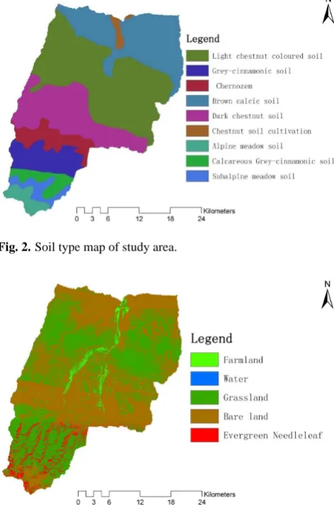
The DHSVM soil data were based on three types of informa-tion: soil type, soil physical parameter (e.g., lateral conduc-tivity, exponential decrease, maximum infiltration, porosity, bubbling pressure, field capacity, wilting point, bulk density) and soil depth. The soil type data was obtained directly from the Chinese 1:1 000 000 soil type classification map, which was interpolated at a spatial resolution of 30 m in Arc/INFO (Fig. 2). Soil physical parameters were defined firstly accord-ing to the FAO global 17-catergory soil physical parameters data and the book “Soil in Xinjiang (Agricultural Bureau of Uygur Autonomous Region of Xinjiang, 1996)”. Table 1 lists some of the soil parameters. Soil depth data were calculated by defining the maximum soil depth (1.3 m) and the mini-mum soil depth (0.25 m) according to observations based on DEM and a program provided by Washington University.

Fig.2 Soil type map of study area

Fig.3 Vegetation classification map of study area Fig. 2. Soil type map of study area.

Fig.2 Soil type map of study area

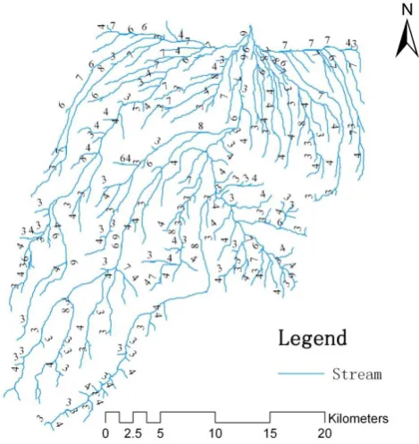
Fig.3 Vegetation classification map of study area Fig. 3. Vegetation classification map of study area.

3.3.3 Vegetation

Five vegetation classes (grassland, farmland, water, bare land and evergreen needle leaf) were derived from Enhanced The-matic Mapper (ETM) classified satellite imagery (Fig.3). Data were processed to be similar in form to the data sets used by Kirschbaum (1997) and Matheussen, et al. (2000). In addition to land classification type, the DHSVM vege-tation parameters (e.g., height, maximum resistance, mini-mum resistance, moisture threshold, vapour pressure deficit, monthly Leaf Area Index (LAI), monthly albedo) were de-fined according to field observation and USGS 25-category vegetation physical parameters. Table 2 lists some of the vegetation parameters.

3.3.4 Snow information

Snow information is very important for stimulating snowmelt runoff, and for the DHSVM model is requires this as an ini-tial snow state file. Snow information included snow cover and spatial distribution of snow water equivalent. In this

Table 1. Suggest examples of soil class and soil parameters.

Soil class Soil parameter

Maximum Porosity Pore Size Bubbling Field Wilting

Infiltration Distribution Pressure Capacity Point

Chernozem 3.0e-5 0.48 0.46 0.46 0.13 0.12 0.12 0.34 0.26 0.26 0.36 0.31 0.31 0.21 0.23 0.23 Brown calcic soil 2.0e-4 0.46 0.48 0.48 0.12 0.13 0.13 0.26 0.34 0.34 0.31 0.36 0.36 0.23 0.23 0.23 Light chestnut coloured soil 1.0e-5 0.39 0.39 0.39 0.12 0.12 0.12 0.29 0.29 0.29 0.27 0.27 0.27 0.17 0.17 0.17 Dark chestnut soil 1.0e-5 0.39 0.46 0.46 0.12 0.12 0.12 0.29 0.26 0.26 0.27 0.31 0.31 0.17 0.23 0.23 Chestnut soil cultivation 1.0e-5 0.46 0.46 0.46 0.12 0.12 0.12 0.26 0.26 0.26 0.31 0.31 0.31 0.23 0.23 0.23 Grey- cinnamonic soil 3.0e-5 0.48 0.49 0.49 0.13 0.10 0.10 0.34 0.34 0.34 0.36 0.37 0.37 0.21 0.25 0.25 Calcareous Grey-cinnamonic soil 1.0e-5 0.46 0.48 0.48 0.12 0.13 0.13 0.26 0.34 0.34 0.31 0.36 0.36 0.23 0.21 0.21 Alpine meadow soil 1.0e-5 0.47 0.47 0.47 0.08 0.08 0.08 0.37 0.37 0.37 0.36 0.36 0.36 0.27 0.27 0.27 Subalpine meadow soil 1.0e-5 0.46 0.46 0.46 0.12 0.12 0.12 0.26 0.26 0.26 0.31 0.31 0.31 0.23 0.23 0.23

paper, the EOS/MODIS data was used to obtain the snow cover information by a normalised difference snow index (NDSI):

NDSI=(Ref4−Ref6)(Ref4+Ref6) (3) Where Ref4, and Ref6is the reflectance of band 4 and band 6 respectively.

Satellite reflectance in MODIS bands 4 and 6 were used to calculate the NDSI for the snow cover map. A pixel is mapped as snow if the NDSI value is>0.4 and the reflectance in MODIS band 2 is>11% (Barton, 2001; Klein, 2003; Sa-lomonson, 2004).

The spatial distribution of snow water equivalent was ob-tained from the National Centre for Atmospheric Research (NCAR) Final analysis data.

3.3.5 Stream network

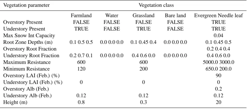
The DHSVM stream network was based on three types of information: a mapping table which located a portion of stream reaches within its appropriate grid cell and described the depth, width, and aspect of the channel cut into the soil; a reach table describing the length, slope, and class of a reach connected with the next reach downstream; and a class file with routing characteristics of width, depth, and roughness for each stream class. These files were derived from the DEM using an algorithm described by Wigmosta and Perkins (2001).

In essence, the DEM topology defines the stream loca-tions, while the extent of the network is specified by the model user via a given support area (minimum area below which a stream channel is assumed to exist). For Juntanghu catchment, the contributing area is 324 000 m2, which was in part based on field observations.

Stream order was used to perform an initial classification of reaches. This produced a manageable number of types

Fig.4 Stream network of Juntanghu basin (Numbers represent the stream order) Fig. 4. Stream network of Juntanghu basin (Numbers represent the stream order).

to which channel characteristics could be indexed. Man-ual adjustments based on limited field observation were con-ducted where necessary (Fig.4). Class characteristics were defined according to field observations (where available) and the relative descriptive size of the classes. The channel depth, width, and roughness were classified according to the reach classifications using GISWA algorithms (Wigmosta and Perkins, 1997). The average slope of each reach was cal-culated using the DEM.

1902 Q. Zhao et al.: A snowmelt runoff forecasting model coupling WRF and DHSVM

Table 2. Suggest parameters of some vegetation classes

Vegetation parameter Vegetation class

Farmland Water Grassland Bare land Evergreen Needle leaf

Overstory Present FALSE FALSE FALSE FALSE TRUE

Understory Present TRUE FALSE TRUE FALSE TRUE

Max Snow Int Capacity 0.04

Root Zone Depths (m) 0.1 0.5 0.5 0.0 0.0 0.0 0.1 0.45 0.4 0.0 0.0 0.0 0.1 0.45 0.5

Overstory Root Fraction 0.2 0.4 0.4

Understory Root Fraction 0.2 0.7 0.1 0.0 0.0 0.0 0.4 0.6 0.0 0.0 0.0 0.0 0.4 0.6 0.0

Maximum Resistance 600 600 5000.0 3000.0

Minimum Resistance 120 200 650.0 200.0

Overstory LAI (Feb.) (%) 90

Understory LAI (Feb.) (%) 0 0 0

Overstory Alb (Feb.) 0.2

Understory Alb (Feb.) 0.12 0.12 0.12

Height (m) 0.8 0.3 20

4 Analysis

4.1 Analyses of forecasting meteorological field results The time period for the case study was from 01:00:00 GMT on 29 February 2008 to 00:00:00 GMT, 6 March 2008.

This study used the WRF with the initial fields and lat-eral boundaries provided by the T213L31 model to realise the 24 h-numerical weather forecast from 29 February 2008 to 6 March 2008. Figure 5 shows the comparative map of ob-served meteorological data and corresponding grid forecasts. From Fig. 5, we can see that: (1) There are certain devi-ations between forecasted and observed temperature at the highest and lowest points. The average error is 1.2 K; (2) The forecasted wind speed is higher than the observed data. This is because WRF only supplies wind speed in every sigma layer, so the wind speed in the lowest sigma layer was adopted. Because the wind speed is a relatively weak influ-ence on the snowmelt runoff and the error is only 1.54 m/s, the forecasted data is acceptable; (3) The relative humidity forecasted error is larger when the humidity fluctuates sig-nificantly. When the relative humidity is stable, the forecast is more accurate. The overall average error is 6%. (4) The forecasted results of solar radiation are generally good. Fore-casted data is significantly higher than observed data at mid-day when the water vapour is higher and cloud activity is greater. It is difficult to consider the effect of clouds due to WRF low spatial resolution.

Overall the forecasting errors are relatively small, proving that limited regional numerical weather forecasting precision can meet the requirements of accurate snowmelt runoff fore-casting.

4.2 Improvement of DHSVM parameters

Hydrology, vegetation and soil parameter schemes have been successfully developed for simulation in North America. A total of 33 parameters were calculated and adjusted in terms of basin climatic and natural conditions. To apply DHSVM model system to snowmelt runoff modelling, the parameter scheme must be improved and reviewed. In this study, all 33 parameters were recalculated and reset by using up-to-date hydrometeorology theory and methodology, focussing on critical parameters such as soil porosity, vertical saturated hydraulic conductivity, maximum infiltration rate and coeffi-cient of roughness for each layer of soil type.

During the spring melt season, there is little Evergreen Needle leaf coverage within the study area. As deciduous foliage is not yet present or is covered by snow, LAI and height of vegetation (except Evergreen Needle leaf) were classifieds as bare land. There are two important soil parameters: Maximum Infiltration rate and Manning’s n which need to be adjusted in snowmelt runoff modelling. (1) Maximum infiltration rate:

Seasonal ground frost is widespread in the catchment dur-ing sprdur-ing melt season. The spatial distribution of frozen soil and snow cover at the start of the spring melt season plays an important role in the generation of spring runoff. Many field studies on snowmelt infiltration into frozen soils have been reported in the literature (Kane and Stein, 1983; Burn, 1991; Gray, Toth and Zhao, 2001; Cherkauer, and Letten-maier, 2003; Niu and Yang, 2006; Zhang and Sun, 2007; Ye, 2009).

Hydrologically, frozen soil suppresses infiltration and encourages surface runoff. In this paper, we empirically hypothesise that as the seasonal frozen soil is distributed

Table 3. The test of forecasted and observed results.

Index Date

29 Feb. 2008 1 Mar 2008 2 Mar 2008 3 Mar 2008 4 Mar 2008 5 Mar 2008

Efficiency coefficient 0.67 0.952 0.912 0.66 0.68 0.96

Relative error of peak runoff 5.19% 2.97% 3.40% 13.2% 11.06% 8.65%

Fig.5 Comparative map of forecasted meteorological data and observed data 260

265 270 275 280 285

2008-2-29 2008-3-1 2008-3-2 2008-3-3 2008-3-4 2008-3-5 Date K Observed temperature

Forecasred temperature

0 1 2 3 4 5 6 7 8 9 10

2008-2-29 2008-3-1 2008-3-2 2008-3-3 2008-3-4 2008-3-5 Date

m/s Observed wind speed

Forecasred wind speed

30 40 50 60 70 80 90

2008-2-29 2008-3-1 2008-3-2 2008-3-3 2008-3-4 2008-3-5 Date % Observed humidity

Forecasred humidity

0 100 200 300 400 500 600 700

2008-2-29 2008-3-1 2008-3-2 2008-3-3 2008-3-4 2008-3-5 Date w/m2 Observed solar radiation

Forecasred solar radiation

Fig. 5. Comparative map of forecasted meteorological data and ob-served data.

under snow cover regions, the maximum infiltration rate of frozen soil is 1.0 e−6_.

(2) Manning’s n:

When compared to the time of energy input at snow sur-face, the delay of snowmelt runoff is due to the water hold-ing capacity of the snowpack and the horizontal travel time of melt water along the ground. This results in a delay in the

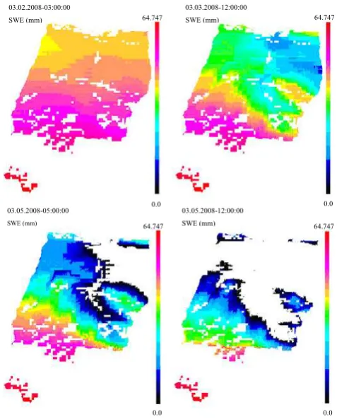
Fig. 6 Spatial change map of snow water equivalent (mm)

03.02.2008-03:00:00 SWE (mm)

03.03.2008-12:00:00 SWE (mm)

03.05.2008-05:00:00

SWE (mm)

03.05.2008-12:00:00 SWE (mm) 64.747

0.0

64.747

0.0

64.747

0.0

64.747

0.0

Fig. 6. Spatial change map of snow water equivalent (mm).

peak time of daily runoff. In this paper the soil parameter, Manning’sn(coefficient of roughness), was adjusted so that the simulated daily flood-peak time matched the observation data.

There is no hydrological and meteorological station in the study area. We have observed the snowmelt process for 3 years (2006, 2007, and 2008). We have observed the daily flood-peak time during the spring melt season in 2006 and 2007. However for the purpose of this study there was insuf-ficient time series runoff data available. Several parameters (e.g., coefficient of roughness, stream network parameters) were adjusted based on observations from 2006 and 2007.

1904 Q. Zhao et al.: A snowmelt runoff forecasting model coupling WRF and DHSVM

1 3 5 7 9 11 13

2008-2-29 2008-3-1 2008-3-2 2008-3-3 2008-3-4 2008-3-5 Date m3/s Observed discharge

Forecasred discharge (With new parameter schemes) Forecasred discharge (With old paramerer schemes)

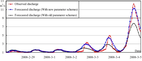
Fig. 7 Comparative map of forecasted discharge and observed discharge

Fig. 7. Comparative map of forecasted discharge and observed dis-charge.

4.3 Analyses of snowmelt runoff results

The DHSVM model was forced by forecasted meteorolog-ical fields at a spatial resolution of 1 km. However, the DHSVM model is initialized at a spatial resolution of 30 m. Therefore there is an interpolated programme embedded within the DHSVM model, which is based on the DEM data (3000) used by WRF model, the high-resolution DEM data (30 m) and temperature gradient. Figure 6 shows the spatial change of snow water equivalent. Figure 7 shows the com-parative map of 24 h-forecasted discharge model with the new model parameter schemes, forecasted discharge with the old model parameter schemes and observed discharge from the outlet of Juntanghu basin from 29 February 2008 to 6 March 2008.

The model efficiency coefficient and the relative error of maximum value are used to evaluate the efficiency of the snowmelt runoff forecasting model. Table 3 shows the test of runoff forecasted with the new model parameter schemes and observed results.

The model efficiency coefficient:

R2=

   

1−

n

P

i=1

(Qobs−Qfore)2 n

P

i=1

Qobs−Qobs

2    

×100% (4)

WhereQobsis the observed discharge (m3/s),Qobsis the average observed discharge (m3/s), Qfore is forecasted dis-charge (m3/s).

The relative error of maximum value:

Rm=

Qobs.m−Qfore.m Qobs.m

(5) WhereQobs.m, andQfore.mis the maximum observed and forecasted discharge (m3/s) respectively.

From Fig. 7 and Table 3, the following results can be ob-served: (1) The average efficiency coefficient is 0.8, which shows the forecasted data is in strong agreement with the observed data. The same trends are present in hydrological processes; and (2) The maximum relative error of maximum

data, which is very important for flood warning, is 13.2%. This means the snowmelt runoff forecasting model is able to meet the needs of snowmelt flood forecasting and flood warning.

5 Conclusion

Based on the latest development of atmospheric science and hydrology, using the features of snowmelt flooding on the northern slopes of Tianshan Mountains, this study has built a snowmelt runoff forecasting model by coupling WRF and DHSVM. The forecasted results of this model have been verified. This was achieved as follows: The limited-region 24-hour Numeric Weather Forecasting System was estab-lished by using the new generation atmospheric model sys-tem WRF2.2 with the initial fields and lateral boundaries pro-vided by the T213L31. Overall, weather predictions were in accordance with observational data. The atmospheric and hydrologic models were coupled and a 24-h snowmelt runoff forecasting model was run using forecasted meteorological fields to force the DHSVM model. With the new parameter schemes taking seasonal ground frost and snow cover into consideration, the simulated data showed strong agreement with the observed data. The average absolute relative error of the maximum runoff in simulation is below 15%. The model has successfully achieved practical snowmelt runoff forecasting.

This study provides safeguards for flood early warning systems, flood prevention and disaster reduction, and water resource management through the forecasting of the meso-microscale snowmelt runoff forecasting model. Coupling the atmospheric and hydrologic models can offer useful refer-ence for hydrological forecasting and water resources man-agement in areas where there is no observed data or incom-plete data.

The results demonstrate the potential of using meso-microscale snowmelt runoff forecasting model for flood fore-casting. The model can provide a longer forecast period compared to traditional models such as those based on rain gauges, or statistical forecasting.

Acknowledgements. The work was supported by a grant from the

Major State Basic Research Development Programme of China (973 Programme) (No. 2007CB411502) and the National Scientific Foundation of China (Nos. 70361001 and 40871023).

This work on meso-microscale snowmelt runoff-forecasting model is an important part of the Project of National Scientific Foundation of China “The decision support system of snowmelt flood warning of Xinjiang based on “3S” technology”.

Edited by: W. Quinton

References

Agricultural Bureau of Uygur Autonomous Region of Xinjiang: Soil Survey Office of Uygur Autonomous Region of Xinjiang: Soil in Xinjiang, Science Press, Beijing, China, 61–752, 1996. Anderson, M. L., Chen Z.-Q., Kawas, M. L., and Feldman, M. L.

A.: Coupling HEC-HMS with atmospheric models for prediction of watershed runoff, J. Hydrologic Engrg., 7(4), 312–318, 2002. Klein, A. G. and Barnett, A. C. : Validation of daily MODIS snow cover maps of the Upper Rio Grande River Basin for the 2000– 2001 snow year, Remote Sens. Environ., 86 162–176, 2003. Barton, J. S., Hall, D. K., and Riggs, G. A.: Thermal and geometric

thresholds in the mapping of snow with MODIS, 11 July, unpub-lished document, 2001.

Ye, B., Yang, D., Zhang, Z., and Kane. D. L.: Variation of hydrolog-ical regime with permafrost coverage over Lena Basin in Siberia, J. Geophys. Res., 114, D07102, doi:10.1029/2008JD010537, 2009.

Burn, C. R.: Snowmelt infiltration into frozen soil at sites in the discontinuous permafrost zone near Mayo, Yukon Territory,in: Northern Hydrology: Selective Perspectives, edited by:: Prowse, T. P and Ommanney, C. S. L., NHRI Symposium No. 6, National Hydrology Research Institute, Environment Canada, Saskatoon, Saskatchewan, 445–459, 1991.

Chen, S. H. and Dudhia, J.: Annual report: WRF physics, Air Force Weather Agency, 38 pp., 2000.

Cherkauer, K. A. and Lettenmaier, D. P.: Simulation of spatial variability in snow and frozen soil, J. Geophys. Res., 108(D22), 8858, doi:10.1029/2003JD003575, 2003.

Gray, D. M., Toth, B., and Zhao, L., et al: Estimating areal snowmelt infiltration into frozen soils, Hydrol. Proc., 15(16), 3095–3111, 2001.

Niu, G. and Yang, Z.: Effects of Frozen Soil on Snowmelt Runoff and Soil Water Storage at a Continental Scale, J. Hydrometeorol., 7(10), 937–952, 2006.

Hong, S. Y., and Pan, H. L.: Nonlocal boundary layer vertical dif-fusion in a medium-range forecast model. Mon. Wea. Rev., 124, 2322–2339, 1996.

Hong, S. Y., Juang, H. M. H., and Zhao, Q.: Implementation of prognostic cloud scheme for a regional spectral model, Mon. Weather Rev., 126, 2621–2639, 1998.

Bartholmes, J. and Todini, E.: Coupling meteorological and hydro-logical models for flood Forecasting, Hydrol. Earth Syst. Sci., 9(4), 333–346, 2005.

Jensen, S. K., and Domingue, J. O.: Extracting topographic struc-ture from digital elevation data for geographic information sys-tem analysis, Photogrammetric Engineering and Remote sensing, 54(11), 1593-1600, 1988.

Kain, J. S., and Fritsch, J. M.: A one-dimensional entraining/ de-training plumes model and its application in convective parame-terization. J. Atmos. Sci., 47, 2784–2802, 1990.

Kain, J. S., and Fritsch, J. M.: Convective parameterization for mesoscale models: The Kain-Fritcsh scheme, The representation of cumulus convection in numerical models, Eedited by: manuel, K. A. and Raymond, D. J., B. Am. Meteor. Soc., 246 pp., 1993. K. E. Saxton, W. J. Rawls, J. S. Romberger, and R. I. Papendick:

Estimating Generalized Soil-water Characteristics from Texture, Soil SCI. SOC. AM. J., 50, 1031–1036, 1986.

Kiamehr, R. and Sjoberg, L. E.: Effect of the SRTM global DEM on the determination of a high resolution geoid model; a case study

in Iran, J. Geod., 79(9), 540–551, 2005.

Kirschbaum, R. and Lettenmaier, D. P.: An evaluation of the effects of anthropogenic activity on streamflow in the Columbia River Basin, Washington, Water Resources Series, Technical Report, University of Washington, Seattle, 156 pp., 1997.

Westrick, K. J. and Mass, C. F.: An Evaluation of a High-Resolution Hydrometeorological Modelling System for Predic-tion of a Cool-Season Flood Event in a Coastal Mountainous Watershed, J. Hydrometeorol., 2, 161–179, 2001.

Li Yan: Change of River Flood and Disaster in Xinjiang during Past 40 Years, J. Glacial. Geocryol., 25(03), 342–346, 2003. Lin, C.A., Wen, L. and B´eland, M.: A coupled

atmospheric-hydrological modelling study of the 1996 Ha! Ha! River basin flash flood in Qu´ebec, Canada, Geophys. Res. Lett., 29, 1026– 1029, doi:10.1029/2001GL013827, 2002.

LU Gui-hua, WU Zhi-yong and LEI Wen: Application of a coupled atmospheric-hydrological modelling system to real-time flood forecast, Advance in Water Science, 6, 847–852, 2006.

Matheussen, B., Kirshbaum, R. L., and Goodman, I. A.: Effects of land cover change on streamflow in the interior Columbia River Basin (USA and Canada), Hydrol. Proc., 14, 867–885, 2000. Michalakes, J., Chen, S., Dudhia, J., and Hart, L.: Development of

a next generation regional weather research and forecast model. In: Developments in Teracomputing: Proceedings of the Ninth ECMWF Workshop on the use of high performance computing in meteorology, Singapore, 269–276, 2001.

Miller, N. L. and Kim, J.: Numerical prediction of precipitation and river flow over the Russian River watershed during the January 1995 storms, B. Am. Meteor. Soc., 77, 101–105, 1996.

Mlawer, E. J., Taubman, S. J., Brown, P. D., Iacono, M. J., and Clough, S. A.: Radiative transfer for inhomogeneous atmo-sphere: RRTM, a validated correlated-k model for the long-wave, J. Geophys. Res., 102(14), 16663–16682, 1997.

Murray, F. W.: On the computation of saturation vapor pressure, J. Appl. Meteorol., 6, 203–204, 1967.

Berry, P. A. M., Garlick, J. D., Smith, R. G.: Near-global validation of the SRTM DEM using satellite radar altimetry, Remote Sens. Environ., 106, 17–27, 2007.

Zhao, Q., Liu, Z., and Shi, Q.: EOS/MODIS data-based estima-tion of the daily snowmelt in Juntanghu Watershed, northern slope of Tianshan Mountain, in: Remote Sensing and Mod-elling of Ecosystems for Sustainability IV, Proc. SPIE, Vol. 6679, 66791C, 2007.

Skamarock, W. C. and Klemp, J. B.: The stability of time-split nu-merical methods for the hydrostatic and the nonhydrostatic elas-tic equations, Mon. Weather Rev., 120, 2109–2127, 1992. Storck, P., and D. P. Lettenmaier, Predicting the effect of a forest

canopy on ground snow accumulation and ablation in maritime climates, in Troendle, C, Ed., Proc. 67th Western Snow Conf., Colorado State University, Fort Collins, 1-12, 1999.

Storck, P.: Trees, snow and flooding: an investigation of forest canopy effects on snow accumulation andmelt at the plot and wa-tershed scales in the Pacific Northwest, Water Resource Series, Technical Report 161, Dept. of Civil Engineering, University of Washington, USA, 2000.

Sun, J. and Zhao, P.: Simulation and analysis of three heavy rain-full processes in 1998 with WRF and MM5, Actameteorological Sinica, 61(6), 692–701, 2003.

Saw-1906 Q. Zhao et al.: A snowmelt runoff forecasting model coupling WRF and DHSVM grass Density, Biomass, and Leaf Area Index: A Flume Study in

Support of Research on Wind Sheltering Effects in the Florida Everglades, Open-File Report 00-172, 2000.

US Department of the Interior, and US Geological Survey: Vegeta-tion ClassificaVegeta-tion for South Florida Natural Areas: Saint Peters-burg, Fl, US Geological Survey, Open-File Report 2006-1240, 1–142, 2006.

USGS: Shuttle Radar Topography Mission (SRTM)—“Finished” Products: U.S. Geological Survey, http://edc.usgs.gov/products/ elevation/srtmbil.html, last date accessed: 30 June 2005. Salomonson, V. V. and Appel, I.: Estimating fractional snow cover

from MODIS using the normalized difference snow index. Re-mote Sensing of Environment, 89 (2004) 351–360.

Wang, W., Barker, D., Bruy ere, C., Dudhia, J.: WRF Version 2 modelling system user’s guide: http://www.mmm.ucar.edu/wrf/ users/docs/userguide/, last access: 2004.

Welsh, P., Wildman, A., Shaw, B., et al.: Implementing the Weather Research and Forecast (WRF) model with local data Assimila-tion in a NWS WFO, 84th AMS Annual Meeting, Seattle, USA, 2004.

Wigmosta, M. S., Vail, L. W., and Lettenamaier, D. P.: A distributed hydrological-vegetation model for complex terrain, Water Re-sour. Res., 30(6), 1665–1679, 1994.

Wigmosta, M. S. and Perkins, W. A.: A GIS-based modelling sys-tem for watershed analysis: Final Report to the National Council of Paper Industry for Arid and Stream Improvement, 1997. Wigmosta, M. S. and Perkins, W. A.: Simulating the effects of

for-est roads on watershed hydrology, in: Influence of Urban and Forest Land Use on the Hydrologic Geomorphic Responses of Watersheds, edited by: Wigmosta, M. S. and Burges, S. J., AGU Water Science and Application Series, 2001.

Rawls, W. J., Nemes, A., Pachepsky, Y. A., and Saxton, K. E.: Us-ing the NRCS National Soils Information System (NASIS) to Provide Soil Hydraulic Properties for Engineering Applications, Am. Soc. Agricult. Biol. Eng., 50(5), 1715–1718, 2007. Wu, S. and Zhang, G.: Preliminary Approach on the Floods

and Their Calamity Changing Tendency in Xinjiang Region, J. Glaciol. Geocryol., 25(2), 199–203, 2003.

Zhang, X., Sun, S., and Xue, Y.: Development and Testing of a Frozen Soil Parameterization for Cold Region Studies, J. Hy-drometeorol., 8(4), 690–701, 2007.

Zhang, F., Ma, X., and Yang, K.: Numerical Simulation and Di-agnostic Analysis of a Heavy Rainfall in Jiangnan Area during 24–25 June 2003. Meteorological Monthly, 30(1), 28–32, 2004.