www.hydrol-earth-syst-sci.net/14/491/2010/ © Author(s) 2010. This work is distributed under the Creative Commons Attribution 3.0 License.
Earth System
Sciences
The Two-layer Surface Energy Balance Parameterization Scheme
(TSEBPS) for estimation of land surface heat fluxes
X. Xin and Q. Liu
State key laboratory of Remote Sensing Science, Institute of Remote Sensing Applications, Chinese Academy of Sciences, Beijing 100101, China
Received: 30 September 2009 – Published in Hydrol. Earth Syst. Sci. Discuss.: 4 November 2009 Revised: 10 February 2010 – Accepted: 9 March 2010 – Published: 12 March 2010
Abstract. A Two-layer Surface Energy Balance
Parameter-ization Scheme (TSEBPS) is proposed for the estimation of surface heat fluxes using Thermal Infrared (TIR) data over sparsely vegetated surfaces. TSEBPS is based on the the-ory of the classical two-layer energy balance model, as well as a set of new formulations derived from assumption of the energy balance at limiting cases. Two experimental data sets are used to assess the reliabilities of TSEBPS. Based on these case studies, TSEBPS has proven to be capable of estimating heat fluxes at vegetation surfaces with acceptable accuracy. The uncertainties in the estimated heat fluxes are comparable to in-situ measurement uncertainties.
1 Introduction
Land surface Evapotranspiration (ET) is one of the most im-portant components in the water cycle between the earth and atmosphere, and plays a very important role in the atmo-sphere, hydroatmo-sphere, and biosphere of the planet. It is an urgent task to understand the evapotranspiration process over different surface types and conditions in agriculture, hydro-geology, forest, and ecology for the purpose of using water resources properly. Additionally, land surface evapotranspi-ration is a key parameter in the synoptic and climatic phe-nomenon because of the heat and moment transfer processes in association with evapotranspiration. Studies (Dickinson, 1984; Avissar, 1998) on climate models and general circula-tion models (GCMs) have found that the climate is sensitive to the change of land surface evapotranspiration. At present, remote sensing may be the only efficient technical way that
Correspondence to: X. Xin (xin [email protected])
can be used to monitor surface evapotranspiration on the re-gional scale (Mu et al., 2007; Stisen et al., 2008). Spatial and temporal distributions of the key state variables of the land surface energy balance can be provided by remote sens-ing, and can be used to estimate surface evapotranspiration. The data of mid-low resolution meteorology and the land re-source satellite can cover large areas of the land surface and can observe repeatedly in short periods, which is useful for the research in the drought monitoring, climate changes, wa-ter resource management, and so on.
Generally, surface evapotranspiration (i.e. latent heat flux LE) is estimated as the residual term of surface energy bal-ance equation. Remotely sensed data have been used suc-cessfully over the past years to estimate the surface net radia-tion and the soil heat flux (hence available energy) from com-bined visible, near infrared and thermal infrared data (Nor-man et al., 1995; Liang et al., 2000; Jacobs et al., 2000; Ma et al., 2002; Ma, 2003). Therefore, the primary focus has been the determination of the sensible heat flux based on the spatially distributed surface temperature fields. The turbulent heat fluxes models to estimate the sensible heat flux can be categorized into two groups, single-source models and dual-source models, according to whether or not the model sepa-rates the foliage and the substrate soil. In the single-source models, a so called “excess” resistance or parameter kB−1 is used to account for the difference between the remotely sensed radiative surface temperatureTrand the aerodynamic
temperature T0 (Moran et al., 1989; Kustas, 1990). The
difference betweenT0 andTr depends on a number of
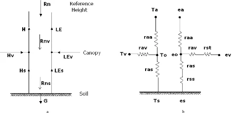
[image:2.595.50.286.64.178.2]
a b
Fig. 1. Energy balance (a) and resistance network (b) of the two-layer model.
Troufleau et al., 1997; Kustas et al., 1999; Massman, 1999) have examined the features of the kB−1 parameter. This parameter is a complex function of canopy structure, water stress and environment factors, and it is too variable to pro-vide a universal solution for estimating the sensible heat flux using single-angle radiative surface temperature. This prob-lem can be circumvented to some extent by using the dual-source models. In this type of models, the heat fluxes of the components (foliage and soil) are simulated individually, and the aerodynamic temperature is analytically expressed in terms of the component temperatures and a set of resistances, as described in the two-layer model proposed by Shuttle-worth and Wallace (1985) and revised by ShuttleShuttle-worth and Gurney (1990). This is very important for sparsely vegetated surfaces, because in this circumstance the contribution of soil surface cannot be neglected. Otherwise, the bias of the esti-mated surface heat fluxes can be significant.
Even though the advantage of the dual-source models in physics has been recognized by the scientific community, the most widely used methods in applications are still based on the assumption of the single source of the surface heat fluxes. This results from such a fact that the use of the two-layer model for operational purpose requires component sur-face temperatures (i.e. soil and vegetation), which is still not available from regular observations and retrieval of the most space-borne remote sensors. Studies of applying the two-layer model with traditional single-angle TIR data have been reported since the model was proposed (Norman et al., 1995; Jupp et al., 1998). Usually, this is achieved by simplifica-tion of the model or adding an empirical relasimplifica-tionship in the model, which decreases the modeling accuracy or limits uni-versal application.
In this study, we have developed a physics-based Two-layer Surface Energy Balance Parameterization Scheme (TSEBPS) for estimation of land surface heat fluxes. We combined the two-layer model developed by Shuttleworth and Wallace (1985) with techniques of handling limiting cases as shown in Su (2002) and Norman et al. (1995) to derive the Component Temperature Dif-ference (CTD) under several extreme soil moisture states.
Additionally, a directional thermal radiative transfer model is used to simulate the radiative surface temperature at these states. Then an index is developed using the observed surface temperature and the simulated temperature at the extreme states. This index is then used to calculate the actual sensible and latent heat fluxes of the foliage and soil surface.
2 TSEBPS (Two-layer Surface Energy Balance Parameterization Scheme)
2.1 The Two-layer Surface Energy Balance model
The classical two-layer model by Shuttleworth and Wal-lace (1985) founded the theory basis for this study (Fig. 1). The surface energy balance is commonly written as
Rn−G=H+LE (1)
WhereRnis the net radiation, Gis the soil heat flux,H is
the sensible heat flux, and LE is the latent heat flux (Lis the latent heat of vaporization andEis the actual evapotranspira-tion). The net radiation of the surface (Rn)can be calculated
from the equation:
Rn=Sd(1−α)+εsLd−Lu (2)
WhereSd are solar irradiation,αsurface albedo, εs surface
emissivity, Ld downward atmosphere long wave radiation,
andLusurface emitted long wave radiation. GCan be
cal-culated with method used by Su (2002):
G=Rn·[0c+(1−fc)·(0s−0c)] (3)
Where,0s=0.315 and0c=0.05, andfcfractional canopy
cov-erage.
The budget of the net radiation between soil and the canopy can be calculated using the Beer’s law:
Rns=b(θ )Rn (4)
Rnv=Rn−Rns (5)
Where Rns and Rnv are the net radiation of soil and the
canopy, andb(θ ) is the gap frequency of the canopy writ-ten as
b(θ )=exp(−G(θ )·LAI/cosθ ) (6)
Where,θis the solar zenith angle, LAI leaf area index of the canopy, andG(θ )projection coefficient of the leaves which is related to the Leaf Angle Distribution (LAD). The energy balance of the soil is written as:
Rns=Hs+LEs+G (7)
The energy balance of the canopy is written as:
The basic principle underlying two-layer models is that the two sources of water vapor and heat are superimposed and hence heat and water vapor enter or leave the bottom layer only via the top one. The total flux of sensible heat emanating from the whole surface is the sum of the fluxes emanating from each layer (here soil and vegetation). So there is
H=Hs+Hv=ρCp
[T0−Ta]
raa
(9) where, ρ is the air density (kg m−3), C
p the specific heat
of air at constant pressure (J kg−1K−1),T0the aerodynamic
temperature (K) defined as the extrapolation of the air tem-perature profile down to the apparent source/sink of heat within the canopy, Ta air temperature (K) at the reference
height, andraathe aerodynamic resistance (s m−1) for heat
transfer. Hs andHv are soil and vegetation sensible heat
fluxes, respectively, which can be expressed according to the gradient-diffusion hypothesis as
Hs=ρCp Ts−T0
ras
(10a)
Hv=ρCp Tv−T0
rav
(10b) Where, Ts andTv are soil and vegetation temperature,
re-spectively,ras the aerodynamic resistance between soil and
the source height in the canopy, andrav the bulk
boundary-layer resistance of the vegetation. The transfer of the latent heat flux in the canopy can also be expressed similarly as: LE=LEs+LEv=
ρCp
γ ·
e0−ea raa
(11)
LEs= ρCp
γ ·
e(Ts)−e0 rss+ras
(12a)
LEv= ρCp
γ ·
e∗(Tv)−e0 rst+rav
(12b)
where,γis the psychometric constant (kPa K−1),e0the
aero-dynamic vapor pressure of the surface,eavapor of the
atmo-sphere, LEs and LEv soil and vegetation latent heat fluxes
respectively,e(Ts)ande∗(Tv)vapor pressure of soil surface
and the saturation vapor pressure in leaf stomata respectively,
rss, andrstsoil surface resistance and leaf stomata resistance
respectively.
Aerodynamic resistanceraais formulated using the
stabil-ity correction method by Choudhury (1989):
raa=ra0φ (13)
Wherera0is the aerodynamic resistance in the neutral
atmo-sphere condition:
ra0=
h
lnz−z d
0
i2
k2u (14)
Whereuis the wind speed at the reference heightz, andk
von Karman’s constant. The corrective termφis calculated with:
φ= 1
(1+η)p
p=2 Stable
p=3/4 Unstable
η=5g(z−d)(T0−Ta)
Tau2
(15)
Where g is acceleration due to gravity (ms−2). The zero
plane displacement height d and the roughness length for momentumz0can be determined following Choudhury and
Monteith (1988), who fitted simple functions to the curves obtained by Shaw and Pereira (1982) from the second-order closure theory:
d=1.1hlnh1+(cdLAI)1/4
i
(16)
z0=
z0s+0.3h(cdLAI)1/2 0≤cdLAI≤0.2
0.3h(1−d/ h) 0.2< cdLAI≤1.5
(17) Where,cd is the mean drag coefficient assumed to be
uni-form within the canopy (0.2), andz0sthe roughness length of
the substrate. For bare soil,z0sis taken as 0.01 m. The
for-mulations for resistancesrasandrav proposed by Choudhury
and Monteith (1988) and Shuttleworth and Gurney (1990) are used here:
rav=αw[w/u(h)]1/2/4α0LAI1−exp(−αw/2) (18)
ras=hexp(αw){exp[−αwz0s/ h] (19)
−exp[−αw(d+z0)/ h]}/[αwK (h)]
Wherew is the leaf width,u(h)the wind speed at canopy heighth,α0andαwtwo constant coefficients equal to 0.005
(ms−1/2) and 2.5 (dimensionless), respectively. The value of
eddy diffusivity at canopy heightK (h) is determined with
K (h)=ku∗(h−d).
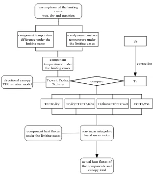
[image:3.595.44.282.422.513.2]2.2 Parameterization scheme based on limiting cases
Figure 2 gives the flow chart of the parameterization. First of all, the limiting cases of soil moisture in the Soil-Plant-Atmosphere Continuum (SPAC) are defined, which are dry-limit, wet-dry-limit, and transition-state. The definitions of the dry- and wet-limit are similar to those in SEBS (Su, 2002), but differ in processing soil and foliage components individu-ally. The transition-state occurs when the surface soil layer is dry and the root zone soil is still wet, which is understandable and predictable in natural vegetation because the drying-off process after a rainfall or irrigation event starts from the sur-face. Then the component temperature difference (CTD, i.e.,
Ts−Tv) at the limiting cases is derived based on the following
assumptions.
correction assumptions of the limiting
cases: wet, dry and transtion
component temperature difference under the
limiting cases
aerodynamic surface temperature under
the limiting cases
component temperatures under
the limiting cases
Tr,wet, Tr,dry,
Tr,trans compare Tr
Tr>Tr,dry Tr,dry>Tr>Tr,tans Tr,thans>Tr>Tr,wet directional canopy
TIR radiative model
Tb
Tr<Tr,wet
non-linear interpolate based on an index component heat fluxes
under the limiting cases
actual heat fluxes of the components and
[image:4.595.140.452.58.415.2]canopy total
Fig. 2. Flow chart of the parameterization scheme of the two-layer models.
moisture and the sensible heat flux is at its maximum value. From Eqs. (1), (7) and (8), it follows,
LEs,dry=0
Hs,dry=Rns−G (20)
and LEv,dry=0 Hv,dry=Rnv
(21) The CTD under this case can be derived from Eq. (10).
δTdry=Ts,dry−Tv,dry=
1
ρCp
[(Rns−G)ras−Rnvrav] (22)
The aerodynamic surface temperature at dry-limitT0,drycan
also be calculated from Eq. (9) based on above assumption. Hence, the soil and foliage temperatures under this caseTs,dry
andTv,drycan be calculated usingδTdryandT0,dry.
Under the wet-limit, where the evaporation and transpi-ration take place at potential rates (i.e. the evapotranspi-ration and transpiration is limited only by the energy available under
the given surface and atmospheric conditions), the sensible heat flux takes its minimum value.
LEwet=LEp (23)
The aerodynamic surface temperature at wet-limitT0,wetcan
be calculated from Eq. (9) based on above assumption. The component temperature difference between soil and foliage can be derived based on the P-M type equation of soil and the canopy and assuming the soil surface resistance and the stomata resistance are zero, we have
Ts,wet=
(Rns−G)ras/ρCp−D0,wet/γ
1+1wet/γ +T0,wet
Tv,wet= Rncrav/ρCp
−D0,wet/γ
1+1wet/γ +T0,wet
δTwet=Ts,wet−Tv,wet= ρC1 p
[(Rns−G)ras−Rncrav] 1+1wet/γ
(24)
whereδTwetis CTD under the wet-limit,1wetis the slope of
the saturation vapor pressure versus the temperature, andγ
is psychrometric constant. Hence, the soil and foliage tem-peratures under this caseTs,wet andTv,wet can be calculated
Under the transition-state, where the evaporation becomes zero due to the limitation of surface soil moisture, and the transpiration is limited only by the energy available (i.e., root zone soil moisture is still at wet-limiting). So there is:
LEs,trans=0 (25)
and the transpiration is simulated using Priestly-Taylor equa-tion.
LEv,trans=a·fg· 1
1+γRnv (26)
where Priestly-Taylor constanta=2.0 according to Kustas et al. (1999),fgis fraction of green leaves in the canopy. So the
aerodynamic surface temperatureT0,transand foliage
temper-atureTv,transunder this case can be calculated using Eqs. (9)
and (10), and the soil temperatureTs,trans under this case is
derived usingT0,transandTv,trans.
Based on the above assumptions and calculations, we have the aerodynamic surface temperature under the limit-ing cases,T0,dry,T0,wet, andT0,trans, and the soil and foliage
temperatures under the limiting cases,Ts,dry,Tv,dry,Ts,trans, Tv,trans, and Ts,wet, Tv,wet. So we also have the sensible
and latent heat fluxes of the soil and foliage under the lim-iting cases,Hs,dry,Hv,dry, LEs,dry, LEv,dry,Hs,trans,Hv,trans,
LEs,trans, LEv,trans, andHs,wet,Hv,wet, LEs,wet, LEv,wetbased
on Eq. (10).
The next step is to derive the actual sensible and latent heat fluxes of the soil and foliage using an interpolation method from the limiting cases. We assume that the dry-and wet-limit cases set reasonable boundaries of the surface heat balance under limiting conditions, and the transition-state gives a key spot where dramatic changes of the bud-get of sensible and latent heat of the canopy take place (i.e., transpiration is at its maximum value and evaporation de-creases between wet-limit and transition-state, and evapora-tion is zero and transpiraevapora-tion decreases between transievapora-tion- transition-state and dry-limit). Increasing or decreasing the soil and foliage heat fluxes can bring about changes in the tempera-tures of the soil and foliage, which can result in canopy sur-face temperature changes. We have derived the component temperatures under the limiting-cases, from which we simu-lated the radiometric surface temperature under the limiting cases,Tr,dry,Tr,wet, andTr,transusing a directional thermal
in-frared radiative transfer model of the canopy. In this study, the model proposed by Franc¸ois (1997) was used to simulate directional radiometric surface temperatures. In the simula-tion, the observing zenith angle takes the actual angle in the field measurement ofTr, and the soil and foliage emissivity
takes the value of 0.94 and 0.98 following Franc¸ois (1997) and Franc¸ois (2002). So the actual heat fluxes can be de-rived based on the comparison between the actual surface temperature and the simulated surface temperature under the limiting-cases.
Comparison between the measured radiometric surface temperature and the simulated surface temperature under the
limiting cases can give a clue of the status of soil moisture, i.e., higher temperature than that under the transition state hints limitation of soil moisture on evaporation, and lower temperature than that under the transition state may indicate relatively better soil moisture condition in the canopy. The derivation of the actual heat fluxes is:
(1) IfTr,wet<Tr<Tr,trans, transpiration is at its maximum
value and evaporation decreases with increasing surface tem-perature, we have:
LEv=LEv,wet=LEv,trans
LEs=(LEs,wet−LEs,trans)·(1−xn)+LEs,trans
(27) wherex is an index build from radiometric surface tempera-tures:
x=(Tr−Tr,wet)/(Tr,trans−Tr,wet) (28)
The sensible heat flux of soil and foliage is then derived as the residual of the energy balance equation of the soil and foliage.
(2) If Tr,trans<Tr<Tr,dry, soil sensible heat flux is at its
maximum value (evaporation is zero) and foliage sensible heat flux increases with increasing surface temperature, we have:
Hs=Hs,dry=Hs,trans
Hv=(Hv,dry−Hv,trans)·(1−yn)+Hv,trans
(29) wherey is an index build from radiometric surface tempera-tures:
y=(Tr,dry−Tr)/(Tr,dry−Tr,trans) (30)
The latent heat flux of soil and foliage is then derived as the residual of the energy balance equation of the soil and fo-liage.
The indicesx andy are used to measure the relative dis-tance of the actual radiometric surface temperatures from the virtual radiometric surface temperatures under the limiting cases. The coefficientnis used to account for the non-linear effect of the heat fluxes changing with the relative change of the surface temperature. Here we take the value ofn=0.25 and it shows that the result is not sensitive to this coefficient. (3) If an unexpected situation happens, such asTr>Tr,dry
orTr<Tr,wet, which may result from the errors of the
mea-surements, simulations and assumptions, the heat fluxes un-der the limiting cases are used for the actual heat fluxes.
3 Data
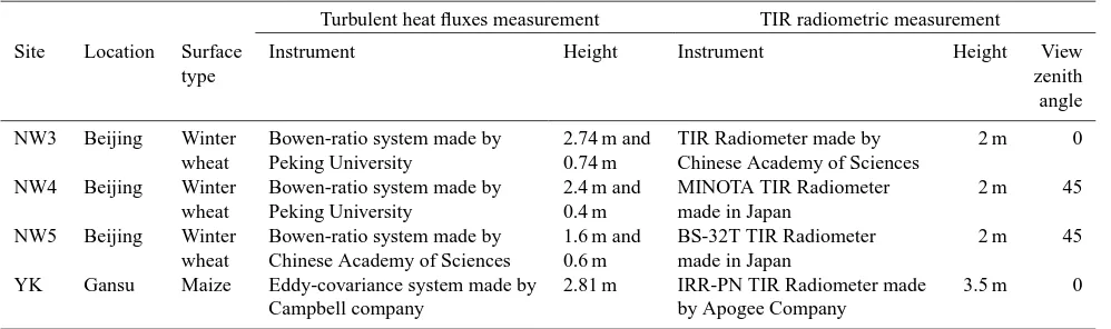
Table 1. Information about the turbulent and TIR measurements.
Turbulent heat fluxes measurement TIR radiometric measurement
Site Location Surface Instrument Height Instrument Height View
type zenith
angle
NW3 Beijing Winter Bowen-ratio system made by 2.74 m and TIR Radiometer made by 2 m 0
wheat Peking University 0.74 m Chinese Academy of Sciences
NW4 Beijing Winter Bowen-ratio system made by 2.4 m and MINOTA TIR Radiometer 2 m 45
wheat Peking University 0.4 m made in Japan
NW5 Beijing Winter Bowen-ratio system made by 1.6 m and BS-32T TIR Radiometer 2 m 45
wheat Chinese Academy of Sciences 0.6 m made in Japan
YK Gansu Maize Eddy-covariance system made by 2.81 m IRR-PN TIR Radiometer made 3.5 m 0
Campbell company by Apogee Company
3.1 Winter wheat in Beijing
The winter wheat dataset was obtained during the “Quanti-tative Remote Sensing theory and application for Land Sur-face Parameters (QRSLSP)” campaign that was carried out in North China in April 2001. The main concern of this ex-periment was for quantitative remote sensing applications in agriculture. The winter wheat fields located in Shunyi dis-trict, north of Beijing (116◦340E, 40◦120N) were selected as the chief observation target. The winter wheat with row structure and regular irrigation is one of the main agricultural crops in North China, and usually the growing period after the winter starts from the end of March through the begin-ning of April. The experiment was carried out in April in or-der to obtain the in-situ data during the rapid growing period of the winter wheat. There are three observation sites, NW3, NW4 and NW5 that are adjacent from south to north, with different planting and management measures, such as wheat cultivar, sowing date, irrigation/fertilization date and amount due to the fields belonging to different farmers, which re-sulted in different surface conditions among the three sites especially the soil moisture. During the experiment period, soil moisture condition was the best in NW4 and the worst in NW5, which resulted in evident difference in heat fluxes and surface temperature between the fields.
Turbulent heat fluxes and meteorological data were measured with Bowen-Ratio (BR) system and Automatic Weather Station (AWS) at the 3 sites, respectively (see Ta-ble 1). The interchange of high- and low-layer measurements takes place for every 10-min for sites NW3 and NW4, and 5-min for site NW5, from which 20-5-min (NW3 and NW4)/10-min (NW5) average turbulent fluxes (H and LE) were com-puted in order to eliminate the discrepancy of equipments at the two sides of the system. 10-min averages of net radiation and soil heat flux were stored. The measured soil heat flux is the value at the 5 cm under the surface for the all sites in this study, and was corrected to the surface by the method of integration using the gradient of soil temperature and the soil
heat flux (Liebethal et al., 2005). In addition, 10-min aver-aged ancillary meteorological data, such as air temperature, relative humidity, and wind speed were also recorded. 10-min average surface brightness temperature was measured and recorded by TIR radiometers, from which the radia-tive surface temperature was obtained by correction of at-mospheric effect and emissivity (Olioso et al., 1996). Hence, every 20-min (NW3 and NW4)/10-min (NW5) averaged heat fluxes, net radiation, soil heat flux, meteorological data, and surface temperature during daytime (when both sensible and latent heat fluxes are positive) were collected as a group of data, and regarded as a sample (see Table 2). The period of available data of the 3 sites are different due to the different beginning/ending time of TIR observation.
As a necessary input for the model, canopy structure data (including Leaf Area Index – LAI, canopy height, leaf shape, and row width and space) were also measured manually by a specific team at the 3 sites regularly during the experiment.
So the winter wheat dataset contains 3 sub-datasets, which represent different soil moisture condition as well as different vegetation density as shown in Table 2. The 3 sub-datasets are used independently to evaluate TSEBPS. More detailed information about the experiment can be found in Liu et al. (2002) for the interested.
3.2 Maize in Gansu
Table 2. Datasets used for the evaluation of TSEBPS.
Dataset Sample number (n) date Leaf Area Index (LAI)
NW3 230 2001-4-1∼22 0.776∼2.402
NW4 188 2001-4-13∼21 2.087∼3.577
NW5 885 2001-4-5∼24 1.028∼3.094
YK-sparse 436 2008-5-21∼6–9 0.24∼0.989
YK-medium 284 2008-6-10∼6–23 1.02∼2.879
YK-dense 368 2008-6-24∼7–15 3.057∼5.298
the irrigation system, which takes the melted snow/ice wa-ter from the upper-stream Qilian mountain area to the flat middle- and lower-stream oasis.
The site Yingke (YK) is located in the artificial oasis to the south of Zhangye city (100◦240E, 38◦510N), where the main crop is maize with row structure and regular irrigation. The turbulent heat fluxes and meteorological data were measured with Eddy-Covariance system (EC) and Automatic Weather Station (AWS). Half-hourly averaged turbulent fluxes (Hand LE) were computed, while 10-min averages of net radiation and soil heat flux were stored. The measured soil heat flux is the value at the 5cm under the surface for the all sites in this study, and was corrected to the surface by the method of integration using the gradient of soil temperature and the soil heat flux (Liebethal et al., 2005). In addition, 10-min av-erage ancillary meteorological data, such as air temperature, relative humidity, and wind speed were also recorded. About 80% energy closure ratio was found in the EC data. Since the two-layer model requires energy conservation, closure in the flux measurements was enforced through a Bowen-ratio method; that is, Bowen-ratio was calculated usingHand LE of the EC measurements, and thenHBR and LEBR were
re-calculated with Bowen-ratio method using net radiation and soil heat flux. 10-min average surface brightness temperature was measured and recorded by TIR radiometers, from which the radiative surface temperature was obtained by correction of atmospheric effect and emissivity (Olioso et al., 1996). Hence, every 30-min averaged heat fluxes, net radiation, soil heat flux, meteorological data, and surface temperature dur-ing daytime (when both sensible and latent heat fluxes are positive) were collected as a group of data, and regarded as a sample (see Table 2). As a necessary input for the surface models, canopy structure data (including leaf area index – LAI, canopy height, leaf shape, and row width and space) were measured manually from 21 May to 15 July throughout the whole growing period before tasseling stage of maize.
Unlike the field campaign of QRSLSP, the experiment of the WATER project had lasted for several months. The data collected during the experiment covers the main grow-ing period of maize, which allows us to evaluate TSEBPS with data of different vegetation coverage states, i.e., from very sparse vegetation at the beginning (LAI<0.5), to very
dense vegetation at the end (LAI>5). In order to evaluate the performance of TSEBPS at different canopy coverage, the dataset of maize was separated into 3 subsets according to LAI; that is YK-sparse for the data when LAI<1.0, YK-medium for 1.0<LAI<3.0, and YK-dense for LAI>3.0.
Table 1 gives the brief information about the turbulent fluxes and TIR radiometric measurements. Table 2 lists the datasets or subsets that are used in the evaluation. In sum-mary, the number of data points is mainly decided by (1) the availability of the observation (because of discontinuity of observation), (2) temporal average of data, (3) processing and quality control of BR and EC data, (4) the data number of daytime (because only the data during daytime when both sensible and latent heat fluxes are positive were used here).
4 Results
The accuracy of TSEBPS will be assessed using the datasets listed in Table 2. Radiative surface temperature as well as ancillary meteorology and canopy structure data were input to the TSEBPS, and the sensible and latent heat fluxes are estimated as discussed previously. All other input variables are measured including net radiation and soil heat flux. The difference between estimation and measurement of the sen-sible and latent heat fluxes will be analyzed for each of the datasets.
4.1 Results of the winter wheat datasets
Sensible heat flux: H
0 50 100 150 200 250 300
0 50 100 150 200 250 300 Simulated (W/m2)
Me
a
su
re
d
(
W
/m
2)
Latent heat flux: LE
0 100 200 300 400 500 600
0 100 200 300 400 500 600 Simulated (W/m2)
Me
a
su
re
d
(
W
/m
2)
a NW3
Sensible heat flux: H
0 50 100 150 200 250
0 50 100 150 200 250
Simulated (W/m2)
Me
a
su
re
d
(
W
/m
2)
Latent heat flux: LE
0 50 100 150 200 250 300 350 400 450 500
0 50 100 150 200 250 300 350 400 450 500 Simulated (W/m2)
Me
a
su
re
d
(
W
/m
2)
b NW4
Sensible heat flux: H
0 50 100 150 200 250 300 350 400
0 50 100 150 200 250 300 350 400 Simulated (W/m2)
Me
a
su
re
d
(
W
/m
2)
Latent heat flux: LE
0 50 100 150 200 250 300
0 50 100 150 200 250 300 Simulated (W/m2)
M
eas
u
re
d
(
W
/m
2)
[image:8.595.129.466.63.515.2]c NW5
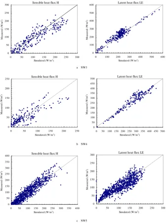
Fig. 3. Comparison between observations and TSEBPS modeled sensible and latentheat fluxes over winter wheat canopy: (a) NW3, (b) NW4, (c) NW5. Dashed line represents perfect agreement.
331.4 and 205.2 Wm−2, respectively. The average value of measured sensible heat flux for the 3 sites is 100.5, 55.4 and 73.4 Wm−2, and the latent heat flux is 224.0, 276.0 and 107.2 Wm−2, respectively. For the latent heat flux, the best agreement appears at NW4, and followed by NW3 and NW5, and all of the predictions are within acceptable accuracy. The data points are scattered closely to the 1:1 line and the bias is confined mostly to within around 50 Wm−2, indicating good
agreement with measured values. There is no obvious trend of overestimate or underestimate of the heat fluxes.
Table 3 to Table 5 show the error statistics of the pre-dicted heat fluxes. Root-Mean-Squared-Error (RMSE), Difference (MAD) and
Table 3. Statistics of TSEBPS estimated versus observed heat fluxes at site NW3 (RMSE: Root Mean Squared Error; MAD: Mean Absolute Deviation; MAPD: Mean Absolute Percentage Deviation;R2: coefficient of determination).
Statistics RMSE MAD MAPD R2 Mean Standard Deviation
(W m−2) (W m−2) (%) (W m−2) (W m−2)
Heat flux estimated measured estimated measured
H 31.4 25.4 25.3 0.8241 113.2 100.5 68.4 60.8
[image:9.595.99.498.224.292.2]LE 31.4 25.4 11.3 0.9046 211.4 224.0 92.8 90.2
Table 4. Statistics of TSEBPS estimated versus observed heat fluxes at site NW4 (RMSE: Root Mean Squared Error; MAD: Mean Absolute Deviation; MAPD: Mean Absolute Percentage Deviation;R2: coefficient of determination).
Statistics RMSE MAD MAPD R2 Mean Standard Deviation
(W m−2) (W m−2) (%) (W m−2) (W m−2)
Heat flux estimated measured estimated measured
H 26.6 20.6 37.4 0.704 54.2 55.4 48.9 39.8
LE 26.6 20.6 7.5 0.9107 277.1 276.0 87.1 88.7
Table 5. Statistics of TSEBPS estimated versus observed heat fluxes at site NW5 (RMSE: Root Mean Squared Error; MAD: Mean Absolute Deviation; MAPD: Mean Absolute Percentage Deviation;R2: coefficient of determination).
Statistics RMSE MAD MAPD R2 Mean Standard Deviation
(W m−2) (W m−2) (%) (W m−2) (W m−2)
Heat flux estimated measured estimated measured
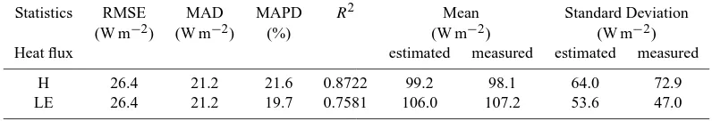
H 26.4 21.2 21.6 0.8722 99.2 98.1 64.0 72.9
LE 26.4 21.2 19.7 0.7581 106.0 107.2 53.6 47.0
fluxes with high accuracy. The highest and lowestR2of the predicted latent heat flux appear at site NW4 and NW5, re-spectively.
In order to investigate the bias of TSEBPS-estimated LE, we compared the relationship between the bias and input parameters and found that the surface temperature gradient (surface temperature minus air temperature) is the mostly re-lated factor with the bias as shown in Fig. 4. We can see that the temperature gradient is mostly under 2 K at NW4, and the bias of estimated LE is also small, mostly within±20 Wm−2.
At point No. 8 (12:00, 13-April), the temperature gradient is the largest (about 8 K), and the bias of estimated LE is also the largest (about−60 Wm−2). At NW5, the temperature gradient is much higher than that of NW4 (mostly between 5∼20 K), and the bias of estimated LE is also larger than that of NW4 (mostly within±50 Wm−2). On the whole, the trend of bias is opposite to that of temperature gradient. Similar to NW4, the points with largest bias (LE was much underesti-mated in Fig. 3) also have very large temperature gradient.
We also investigated the correlation between the bias of TSEBPS-estimated LE and wind speed. It can be seen from Fig. 4 that there is no obvious trend in the correlation for
[image:9.595.98.496.348.416.2]Table 6. Statistics of TSEBPS estimated versus observed heat fluxes at site YK (RMSE: Root Mean Squared Error; MAD: Mean Absolute Deviation; MAPD: Mean Absolute Percentage Deviation;R2: coefficient of determination).
Statistics RMSE MAD MAPD R2 Mean Standard Deviation
(W m−2) (W m−2) (%) (W m−2) (W m−2)
Heat flux estimated measured estimated measured
H 31.0 23.7 32.3 0.7610 79.9 73.4 56.0 61.8
LE 31.0 23.7 9.0 0.9722 255.5 262.0 169.9 178.2
-80 -60 -40 -20 0 20 40 60 80
1 10 19 28 37 46 55 64 73 82 91 100 109 118 127 136 145 154 163 172 181
data point error of esti mate d LE ( W/m2 ) -6 -4 -2 0 2 4 6 8 10 Tr-T a(K) or U a (m /s) bias dT Ua NW4 -100 -75 -50 -25 0 25 50 75 100
1 51 101 151 201 251 301 351 401 451 501 551 601 651 701 751 801 851
data point e rr or of es tim at ed LE (W /m2 ) 0 5 10 15 20 25 30 T r-Ta (K ) o r U a (m/ s) bias dT Ua NW5 -80 -60 -40 -20 0 20 40 60 80
1 10 19 28 37 46 55 64 73 82 91 100 109 118 127 136 145 154 163 172 181
data point error of esti mate d LE ( W/m2 ) -6 -4 -2 0 2 4 6 8 10 Tr-T a(K) or U a (m /s) bias dT Ua NW4 -100 -75 -50 -25 0 25 50 75 100
1 51 101 151 201 251 301 351 401 451 501 551 601 651 701 751 801 851
data point e rr or of es tim at ed LE (W /m2 ) 0 5 10 15 20 25 30 T r-Ta (K ) o r U a (m/ s) bias dT Ua NW5
Fig. 4. Time series of TSEBPS estimated latent heat flux bias (TSEBPS estimated minus measured latent heat flux) versus surface temperature gradient (radiative surface temperature minus air temperature) and wind speed.
4.2 Results of the maize dataset
The canopy sensible and latent heat fluxes predicted versus the measured values are shown in Fig. 5. Similar to the win-ter wheat dataset, the estimated sensible and latent heat fluxes agree very well with the measurement. Table 6 shows the er-ror statistics of the predicted heat fluxes. The average value of available energy (net radiation minus soil heat flux), sen-sible and latent heat fluxes is 335.4, 73.4 and 262.0 Wm−2, respectively. RMSE and MAPD of the estimated latent heat flux are low and the coefficient of determination (R2) is very high, which means that the TSEBPS-estimated latent heat flux with TIR measurements can reach high accuracy. Mean and standard deviation of the predicted heat fluxes compare very well with those measured as shown in Table 6.
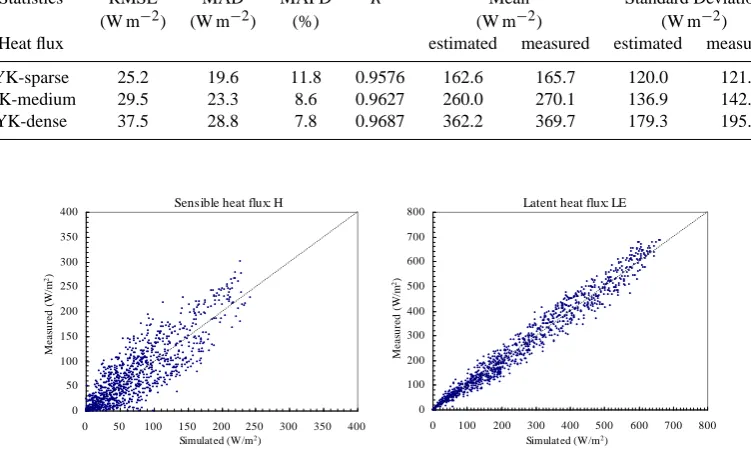
In order to investigate the performance of TSEBPS at different vegetation coverage conditions, the error statistics are recalculated separately for the 3 subsets of the maize
according to Table 2. The results are shown in Table 7, from which we can see that there is no evident difference in the
R2 between the subsets, but the RMSE shows much more variability between the subsets, i.e., RMSE increases with increasing LAI. On the other hand, MAPD decreases with increasing LAI. Comparison of mean and standard deviation shows that datasets of medium and dense canopy have larger bias than that of sparse canopy. However, the difference between the subsets is not evident, and the performance of TSEBPS is stable from very sparse to very dense canopies. It means that TSEBPS can estimate heat fluxes accurately above surfaces with different density of vegetation.
Table 7. Statistics of TSEBPS estimated versus observed heat fluxes at three different growing stages of maize at site YK (RMSE: Root Mean Squared Error; MAD: Mean Absolute Deviation; MAPD: Mean Absolute Percentage Deviation;R2: coefficient of determination).
Statistics RMSE MAD MAPD R2 Mean Standard Deviation
(W m−2) (W m−2) (%) (W m−2) (W m−2)
Heat flux estimated measured estimated measured
YK-sparse 25.2 19.6 11.8 0.9576 162.6 165.7 120.0 121.5
YK-medium 29.5 23.3 8.6 0.9627 260.0 270.1 136.9 142.7
YK-dense 37.5 28.8 7.8 0.9687 362.2 369.7 179.3 195.0
Sensible heat flux: H
0 50 100 150 200 250 300 350 400
0 50 100 150 200 250 300 350 400 Simulated (W/m2)
Me
a
su
re
d
(
W
/m
2)
Latent heat flux: LE
0 100 200 300 400 500 600 700 800
0 100 200 300 400 500 600 700 800 Simulated (W/m2)
Me
a
su
re
d
(
W
/m
2)
Fig. 5. Comparison between observations and TSEBPS modeled sensible and latentheat fluxes over maize canopy. Dashed line represents perfect agreement.
Nevertheless, it is hard to compare the different measure-ment techniques based on the present datasets and give a con-clusion about the uncertainties of the measurements in this study. Fortunately, some useful information can be found in the references that analyzed the variation of flux estima-tion by various micrometeorological techniques based on the datasets obtained in other experiment projects, such as Mon-soon’90, FIFE, and ChinaFLUX (Norman et al., 1995; Twine et al., 2000; Massman et al., 2002; Yu et al., 2006). Accord-ing to the references and other studies that compare model predicted flux with in-situ measurements (e.g., Timmermans et al., 2007), uncertainties of fluxes are about 25∼50 Wm−2
for H and LE measured by EC technique, and about 20% for LE measured by BR technique. The errors of TSEBPS-estimated heat fluxes are of similar magnitude with the un-certainties in the measurements, which means that TSEBPS is able to predict surface heat fluxes with acceptable accu-racy.
4.3 Error analysis
According to the flow chart of TSEBPS (Fig. 2), the actual heat fluxes are derived from the heat fluxes of the limiting cases with an interpolating method. So the error of TSEBPS-estimated heat fluxes comes from these two aspects, i.e., the heat fluxes of the limiting cases and the interpolating meth-ods. The sensitivity of the estimated heat flux to the error of
the heat flux at the limiting cases is described by the follow-ing way.
1Y =Y (Yi±0.1Yi)−Y (Yi)
Y (Yi)
(31) whereY represents the derived actual heat flux, and Yi the
heat flux at the limiting cases (i.e., wet- and dry-limits, and transition state). From Eqs. (27) and (29), we can see that the non-linear interpolation takes place for soil latent heat flux when Tr,wet<Tr<Tr,trans, and for foliage sensible heat flux
whenTr,trans<Tr<Tr,dry. And at other cases, the interpolation
is linear. Sensitivity to the error of LEs,wetin Eq. (27) and the
error ofHv,dryin Eq. (29) can be expressed in a same way:
1Y = ± 1
10+ 10Apn
1−pn
(32)
whereArepresents LEs,trans/LEs,wetandpforxfor Eq. (27),
andA representsHv,trans/Hv,dry andp for y for Eq. (29).
According to the assumption of TSEBPS (Eqs. 25 and 26),
Aequals to 0 or is very close to 0 (no negative value of the heat fluxes is allowed in the calculation), which results in that the sensitivity to the error of LEs,wetandHv,dryis nearly
[image:11.595.107.483.109.334.2]Sensitivity to the error of LEs,transin Eq. (27) and the error
ofHv,transin Eq. (29) can also be expressed in a same way:
1Y = ± 1
10+10(1−pn)
Apn
(33)
BecauseAequals to 0 or is very close to 0, the sensitivity to the error of LEs,trans andHv,trans is very small and can
be regarded as 0. It means that the error of component heat fluxes at the transition state has no obvious influence on the estimated heat fluxes.
Sensitivity to the error ofp(x in Eq. 27 andy in Eq. 29) can be expressed as:
1Y =1−(1±0.1)
n
1
(1−A)pn −1
(34)
BecauseAequals to 0 or is very close to 0, the sensitivity to the error ofp mainly varies with p. The magnitude of
p is within the range of [0, 1]. Whenp is close to 0, the sensitivity is small, and whenpis close to 1, the sensitivity becomes relatively larger. And the sign of the error in the estimated heat fluxes is opposite to that ofp. In our datasets, the average value ofpis about 0.5∼0.6, which leads to about ±10∼20% error in the estimated heat fluxes for ±10% of error inp.
From above analysis we can see that±10% error in the component heat fluxes at the wet- and dry-limiting cases will result in about±10% error in TSEBPS- estimated heat fluxes, and the error in the component heat fluxes at the tran-sition state will result in no obvious error in TSEBPS- es-timated heat fluxes. The component heat fluxes at the lim-iting cases are calculated using Eq. (10) with the aerody-namic temperature and component temperatures, which are calculated based on the assumptions of the limiting cases. In this study, the assumptions and calculations are physics-based and the error in the estimated component heat fluxes is regarded within acceptable range.
On the other hand, the error in the simulated surface tem-perature at the limiting cases has obvious influence on the results. The error ofpcomes from the error of TIR observa-tion, as well as the error of the simulated surface temperature at the limiting cases. In our study, a directional canopy TIR radiation transfer model by Franc¸ois (1997) is used to simu-late the surface temperature at the limiting cases. This model is of reasonable physics-basis and has performed well in the experimental study in the reference. In their study, the error of the simulated temperature is relatively small and accept-able. In this study, we believe that the simulated temperature is of good quality and comparable to the field TIR observa-tion. Furthermore, from Eqs. (28) and (30) we can see that the error inxandycan be relatively small because the index is constructed by the difference between the temperatures, which means that the error of the temperature can wipe one another out.
At last, some may argue that the error may come from the coefficientn. This coefficient is empirical and we took
n=0.25 because it gives the best accuracy in the results. And this value is identical for both winter wheat and maize datasets, which implies that the coefficient may have a uni-versal value for all of the surfaces, but this still needs to be proved by more investigations.
5 Discussions
TSEBPS is proposed to estimate surface heat fluxes using TIR data obtained by space-borne sensors such as AVHRR, MODIS, etc. This kind of data is easily available and eco-nomical for the users, which is important for applications at regional or global scale with routinely schedule. For re-gional or global estimation of land surface evapotranspira-tion, sparsely vegetated surface is one of the situations of relatively larger uncertainty, where single layer model as-sociated with TIR data can not simulate the canopy heat fluxes accurately. As a parameterization of the classical two-layer model, TSEBPS is reliable on the theory basis. It was shown in the evaluation using datasets over different veg-etation canopies that TSEBPS-estimated evapotranspiration compared very well with the field measurement. The param-eterization is based on the limiting cases of soil moisture, which is commonly accepted. The difference of TSEBPS is to consider foliage and soil independently at the limiting cases, and bring a key state of soil moisture into the model, i.e., transition state, which is based on the process of dry-ing off after a rain or irrigation event when the soil surface is dry and the root zone is still wet. By the concept of tran-sition state, we can hence define two different states of soil moisture in the canopy, i.e., before and after the transition, which represent the limit of soil moisture is only on Evapo-ration (E) or on both EvapoEvapo-ration (E) and TranspiEvapo-ration (T). The canopy heat fluxes are then easily predictable using the assumptions of the limiting cases associated with an interpo-lation method using TIR data. Commonly, all of the states of soil moisture can be described by such assumptions. How-ever, there are exceptions when the soil surface is wet and root zone is relatively drier, which could be possible when there is heavy dew or light precipitation while the field has been under drought already. Under this circumstance, the relationship between surface temperature and soil moisture would be different from the assumption of TSEBPS, and TSEBPS-estimated heat fluxes would be of substantial error. Fortunately, this kind of exception is not a frequent event, i.e., once or twice during the whole growing season of crop, which will not affect the applicability of TSEBPS in the long term.
heat fluxes is able to produce good results and can be used widely for surfaces with different soil moisture and vegeta-tion condivegeta-tions.
According to the sensitivity analysis, the TSEBPS-estimated heat fluxes are not sensitive to the assumed heat fluxes at the limiting cases as well as the error of the sim-ulated temperature. On the other hand, it was found that higher accuracy can be obtained by using more complex model to allocate net radiation into soil and foliage. How-ever, this could restrict the applicability of TSEBPS in satel-lite data. Compromise between accuracy and convenience has to be made. Fortunately, a simple method such as shown in Eqs. (4) to (6) can calculate soil and foliage net radiation reasonably and result acceptable heat fluxes in this study. On this meaning, the method proposed and used in this study is applicable for regional estimation of ET using satellite data. Results of evaluation of TSEBPS using satellite data will be reported by the authors in the near future.
6 Conclusions
Two-layer energy balance model has been validated and ap-proved at many references. However, its application in re-mote sensing is still of problem because of short of com-ponent temperatures data. In this study, a parameteriza-tion scheme (TSEBPS) was proposed to utilize the two-layer model with traditional TIR observation data. The parameter-ization is based on the assumption of the changing process of sensible and latent heat fluxes of the foliage and sub-layer soil with the change of soil moisture at surface layer and root zone. The actual canopy heat fluxes are derived from the ob-served radiative surface temperature by comparing with the simulated temperatures at the limiting cases. Two datasets obtained in two different field experiments were used to eval-uate the reliability of TSEBPS. The estimated canopy heat fluxes agreed well with the field measurements of heat fluxes. The uncertainties of the estimation are comparable to in-situ measurement uncertainties. The errors of TSEBPS mainly come from the following aspects, i.e., the assumption of the limiting cases, and the interpolation method of heat fluxes using the TIR observations. Although extensive evaluation should be carried out using more in-situ or remotely sensed data, the results of this study showed that the method pro-posed in this paper is reliable and can be used to estimate heat fluxes over sparsely vegetated surfaces.
Acknowledgements. This work was carried out under the aus-pices of Chinese Natural Science Fund Project (40601067), the Knowledge Innovation Project of Chinese Academy of Sciences (KZCX2-YW-313), China’s Special Funds for Major State Basic Research Project (2007CB714402), Chinese Natural Science Fund Project (40730525), the Special Research Foundation of
Public Benefit Industry (GYHY200706046-1), and Youth Research Foundation of IRSA (08S01200CX).
Edited by: X. W. Li
References
Avissar, R.: Which type of SVAT is needed for GCMs, J. Hydrol., 50, 3751–3774, 1998.
Bastiaanssen, W. G. M., Menenti, M., Feddes, R. A., and Holtslag, A. A. M.: A remote sensing surface energy balance algorithm for land (SEBAL), J. Hydrol., 212–213, 198–212, 1998.
Blyth, E. M. and Dolman, A. J.: The roughness length for heat of sparse vegetation, J. Appl. Meteorol., 34, 583–585, 1995. Brutsaert, W.: Evaporation into the Atmosphere, Reidel, Dordrecht,
Netherlands, 299 pp., 1982.
Caselles, V., Sobrino, J. A., and Coll, C.: A physical model for inter-preting the land surface temperature obtained by remote sensing sensors over incomplete canopies, Remote Sens. Environ., 39, 203–211, 1992.
Chehbouni, A., Lo Seen, D., Njoku, E. G., and Monteny, B. M.: Ex-amination of the difference between radiative and aerodynamic surface temperatures over sparsely vegetated surfaces, Remote Sens. Environ., 58, 177–186, 1996.
Chehbouni, A., Nouvellon, Y., Lhomme, J. P., Watts, C., Boulet, G., Kerr, Y. H., Moran, M. S., and Goodrich, D. C.: Estimation of surface sensible heat flux using dual angle observations of ra-diative surface temperature, Agr. Forest Meteorol., 108, 55–65, 2001.
Choudhury, B. J.: Estimating evaporation and carbon assimilation using infrared temperature data: vistas in modeling, in: Theory and Applications of Remote Sensing, edited by: Asrar, G., John Wiley, New York, 628–690, 1989.
Choudhury, B. J. and Monteith, J. L.: A four-layer model for the heat budget of homogeneous land surfaces, Q. J. Roy. Meteor. Soc., 114, 373–398, 1988.
Choudhury, B. J., Reginato, R. J., and Idso, S. B.: An analysis of infrared temperature observations over wheat and calculation of latent heat fluxes, Agr. Forest Meteorol., 37, 75–88, 1986.
Dickinson, R. E.: Modeling evapotranspiration for
three-dimensional global climate models, in Climate Processes and Climate Variability, edited by: Hanson, J. E. and Takahashi, T., Am. Geophys. Union, 58–72, 1984.
Franc¸ois, C.: The potential of directional radiometer temperatures for monitoring soil and leaf temperature and soil moisture status, Remote Sens. Environ., 80, 122–133, 2002.
Franc¸ois, C., Ottl´e, C., and Pr´evot, L.: Analytical parameterization of canopy directional emissivity and directional radiance in the thermal infrared, Application on the retrieval of soil and foliage temperatures using two directional measurements, Int. J. Remote Sens., 18, 2587–2621, 1997.
Friedl, M. A.: Modeling land surface fluxes using a sparse canopy model and radiometric surface temperature measurements, J. Geophys. Res., 100, 25435–25446, 1995.
Jacobs, J. M., Myers, D. A., Anderson, M. C., and Diak, G. R.: GOES surface insolation to estimate wetlands evapotranspira-tion, J. Hydrol., 266, 53–65, 2000.
Jupp, D. L. B., Tian, G., McVicar, T. R., Qin, Y., and Li, F.: Soil moisture and drought monitoring using remote sensing I: Theo-retical background and methods, EOC Report1, 16–21, 1998. Kimes, D. S.: Remote sensing of row crop structure and component
temperatures using directional radiometric temperatures and in-version techniques, Remote Sens. Environ., 13, 33–55, 1983. Kustas, W. P.: Estimates of evapotranspiration with a one- or
two-layer model of heat transfer over partial canopy cover, J. Appl. Meteorol., 29, 704–715, 1990.
Kustas, W. and Jackson, T.: The impact on area-averaged heat fluxes from using remotely sensed data at different resolutions: a case study with Washita’92 data, Water Resour. Res., 35, 1539– 1550, 1999.
Lhomme, J. P., Monteny, B., and Amadou, M.: Estimating sensible heat flux from radiometric temperature over sparse millet, Agr. Forest Meteorol., 68, 77–91, 1994.
Li, F., Kustas, W. P., Prueger, J. H., Neale, C. M. U., and Jackson, T. J.: Utility of remote sensing based two-source energy balance model under low and high vegetation cover conditions, J. Hy-drometeorol., 6, 878–891, 2005.
Li, X., Li, X. W., Li, Z. Y., Ma, M. G., Wang, J., Xiao, Q., Liu, Q., Che, T., Chen, E. X., Yan, G. J., Hu, Z. Y., Zhang, L. X., Chu, R. Z., Su, P. X., Liu, Q. H., Liu, S. M., Wang, J. D., Niu, Z., Chen, Y., Jin, R., Wang, W. Z., Ran, Y. H., Xin, X. Z., and Ren, H. Z.: Watershed Allied Telemetry Experimental Research, J. Geophys. Res., 114, D22103, doi:10.1029/2008JD011590, 2009.
Liang, S. L.: Narrowband to broadband conversions of land sur-face albedo: I Algorithms, Remote Sens. Environ., 76, 213–238, 2000.
Liang, S.L., Stroeve, J. C., Grant, I. F., Strahler, A. H., and Duvel, J. P.: Angular Corrections to Satellite Data for Estimating Earth Radiation Budget, Remote Sens. Rev., 18, 103–136, 2000. Liebethal, C., Huwe, B., and Foken, T.: Sensitivity analysis for two
ground heat flux calculation approaches, Agr. Forest Meteorol., 132, 253–262, 2005.
Liu, Q., Liu, Q. H., Xiao, Q., and Tian, G. L.: Study on geometric correction of airborne multi-angular imagery, Sci. China Ser. D, 45(12), 1075–1086, 2002.
Liu, Q. H., Liu, Q., and Xin, X. Z.: Experiment study of direc-tional radiance and hotspot effect in thermal infrared observation of corn canopy, Proc. IGARSS’01, Sydney, Australia, 2001. Liu, Q. H., Li, X. W., Chen, L. F., and 973 Project Members: Field
Campaign for Quantitative Remote Sensing in Beijing, J. Remote Sens., 6(Suppl.), 43–49, 2002.
Ma, Y., Su, Z., Li, Z., Koike, T., and Menenti, M.: Determination of regional net radiation and soil heat flux over a heterogeneous landscape of the Tibetan Plateau, Hydrol. Process., 16, 2963– 2971, 2002.
Ma, Y. M.: Remote sensing parameterization of regional net radia-tion over heterogeneous land surface of Tibetan Plateau and arid area, Int. J. Remote Sens., 24, 3137–3148, 2003.
Massman, W. J.: A model study of kB−H1for the vegetated surfaces using “localized near-field” Lagrangian theory, J. Hydrol., 223, 27–43, 1999.
Massman, W. J. and Lee, X.: Eddy covariance flux corrections and uncertainties in long term studies of carbon and energy ex-changes, Agr. Forest Meteorol., 113, 121–144, 2002.
Moran, M. S., Jackson, R. D., Raymond, L. H., Gay, L. W. and Slater, P. N.: Mapping surface energy balance components by combining Landsat thematic mapper and ground-based meteoro-logical data, Remote Sens. Environ., 30, 77–87, 1989.
Mu, Q., Heinsch, F. A., Zhao, M., and Running, S. W.: Develop-ment of a global evapotranspiration algorithm based on MODIS and global meteorology data, Remote Sens. Environ., 111, 519– 536, 2007.
Norman, J. M., Kustas, W. P., and Humes, K. S.: Source approach for estimating soil and vegetation energy fluxes in observations of directional radiometric surface temperature, Agr. Forest Me-teorol., 77, 263–293, 1995.
Olioso, A., Taconet, O., and Mehrez, M. B.: Estimation of heat and mass fluxes from IR brightness temperature, IEEE T. Geosci. Remote, 34, 1184–1190, 1996.
Shaw, R. H. and Pereira, A. R.: Aerodynamic roughness of a plant canopy: a numerical experiment, Agr. Forest Meteorol., 26, 51– 65, 1982.
Shuttleworth, W. J. and Wallace, J. S.: Evaporation from sparse crops – an energy combination theory, Q. J. Roy. Meteor. Soc., 111, 839–855, 1985.
Shuttleworth, W. J. and Gurney, R. J.: The theoretical relation-ship between foliage temperature and canopy resistance in sparse crop, Q. J. Roy. Meteor. Soc., 116, 497–519, 1990.
Sobrino, J. A. and Caselles, V.: Thermal infrared radiance model for interpreting the directional radiometric temperature of a veg-etative surface, Remote Sens. Environ., 33, 193–199, 1990. Stisen, S., Sandholt, I., Nørgaard, A., Fensholt, R., and Jensen, K.
H.: Combining the triangle method with thermal inertia to es-timate regional evapotranspiration – Applied to MSG-SEVIRI data in the Senegal River basin, Remote Sens. Environ., 112, 1242–1255, 2008.
Su, Z.: The surface energy balance system (SEBS) for estimation of turbulence heat fluxes, Hydrol. Earth Syst. Sc., 6(1), 85–99, 2002.
Timmermans, W., Kustas, W., Anderson, M., and French, A.: An intercomparison of the Surface Energy Balance Algorithm for Land (SEBAL) and the Two-Source Energy Balance (TSEB) modeling schemes, Remote Sens. Environ., 108(4), 369–384, 2007.
Troufleau, D., Lhomme, J. P., Monteny, B., and Vidal, A.: Sensi-ble heat fluxes and radiometric temperature over sparse Sahelian vegetation: I. An experimental analysis of thekB−1parameter, J. Hydrol., 188–189, 815–838, 1997.
Twine, T. E., Kustas, W. P., Norman, J. M., Cook, D. R., Houser, P. R., Meyers, T. P., Prueger, J. H., Starks, P. J., and Wesely, M. L.: Correcting eddy-covariance flux underestimates over a grass land, Agr. Forest Meteorol., 103, 279–300, 2000.
Verhoef, A., de Bruin, H. A. R., and van den Hurk, B. J. J. M.: Some practical notes on the parameter for sparse vegetation, J. Appl. Meteorol., 36, 560–572, 1997.