State space approach to evaluate spatial variability of field measured soil water status along a line transect in a volcanic vesuvian soil

www.hydrol-earth-syst-sci.net/14/2455/2010/ doi:10.5194/hess-14-2455-2010

© Author(s) 2010. CC Attribution 3.0 License.

Earth System

Sciences

State-space approach to evaluate spatial variability of

field measured soil water status along a line transect in

a volcanic-vesuvian soil

A. Comegna1, A. Coppola1, V. Comegna1, G. Severino2, A. Sommella2, and C. D. Vitale3

1_{Department for Agro-Forestry Systems Management (DITEC), Hydraulics Division,} University of Basilicata, Potenza, Italy

2_{Division of Water Resources Management, University of Naples “Federico II”, Italy} 3_{Department of Economics and Statistical Sciences , University of Salerno, Italy}

Received: 14 July 2010 – Published in Hydrol. Earth Syst. Sci. Discuss.: 1 September 2010 Revised: 22 November 2010 – Accepted: 23 November 2010 – Published: 7 December 2010

Abstract. Unsaturated hydraulic properties and their spatial

variability today are analyzed in order to use properly math-ematical models developed to simulate flow of the water and solute movement at the field-scale soils. Many studies have shown that observations of soil hydraulic properties should not be considered purely random, given that they possess a structure which may be described by means of stochastic pro-cesses. The techniques used for analyzing such a structure have essentially been based either on the theory of regional-ized variables or to a lesser extent, on the analysis of time series. This work attempts to use the time-series approach mentioned above by means of a study of pressure headhand water contentθ which characterize soil water status, in the space-time domain. The data of the analyses were recorded in the open field during a controlled drainage process, evap-oration being prevented, along a 50 m transect in a volcanic Vesuvian soil. The isotropic hypothesis is empirical proved and then the autocorrelation ACF and the partial autocorre-lation functions PACF were used to identify and estimate the ARMA(1,1) statistical model for the analyzed series and the AR(1) for the extracted signal. Relations with a state-space model are investigated, and a bivariate AR(1) model fitted. The simultaneous relations betweenθandhare considered and estimated. The results are of value for sampling strate-gies and they should incite to a larger use of time and space series analysis.

Correspondence to: A. Comegna ([email protected])

1 Introduction

The increasing need for water for domestic and industrial purposes under ever more stringent environmental protec-tion measures, combined with advances in irrigaprotec-tion, makes it necessary to gain in-depth knowledge of water and solute flow in the vadose zone, understood as the zone roughly ex-tending from the soil surface to the water table. Mathemati-cal models have for some time been available that allow the probable losses of water by evaporation and percolation to be estimated, as well as the probable solute residence times and the evolution of available water reserves (Feddes et al., 1988). Based on laws of water flow in unsaturated porous media, in order to be applied such models are known to re-quire mathematical relations linking the local value of water content in volumeθto the water tensionhand soil hydraulic conductivityk. Experimental observations to measure as di-rectly as possible the relations between θ, hand k can be developed through field trials (Hillel, 1998). It is also well known that in field applications of models, to achieve re-sults of a practical interest, there must be an evaluation in statistical terms of the variability of such observable parame-ters also in fairly homogeneous natural media. Deterministic evaluation of spatial heterogeneity of soil physical and hy-draulic properties requires a large number of measurements and hence can only be performed for limited areas. This has led to the increasing use of statistical models in which hy-draulic variables are considered stochastic (Freeze, 1975).

2456 A. Comegna et al.: State-space approach to evaluate spatial variability

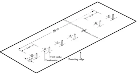
Fig. 1. View of the experimental plot displaying relative position of TDR probes and 0.3 m depth tensiometers.

observations concerning the property in question as statisti-cally independent quantities abstracted from their spatial po-sition. Only in recent years have surveys been conducted that have clearly shown the existence of a spatial structure of heterogeneities (Russo and Bresler, 1981). This structure has been described with geostatistical techniques essentially derived from regionalized variable theory (Matheron, 1971) in terms of semivariograms. Each physical property, in the case of isotropy, could thus be considered as the realization of a stochastic process which is a function of coordinates on a horizontal plane and, in the case of anisotropy, a function of direction. Applications of such techniques have proved promising for describing variability in space of soil hydraulic properties and have led to defining the number and distance at which to make determinations, thereby reducing sampling costs (Vieira et al., 1981).

Another group of techniques, also used to study the structure of variability, is based on a modified time se-ries theory (Box and Jenkins, 1970). By using such tech-niques, the structure may be described in terms of auto-correlation functions and SARMA (Spatial Autoregressive-Moving Average) models with a view to estimating the stochastic properties of the data. Some of these applica-tions in soil physics and hydrology include the studies by Morkoc et al. (1985), Anderson and Cassel (1986), Wen-droth et al. (1992), Cassel et al. (2000), Heuvelink and Web-ster (2001), Wendroth et al. (2006).

In the present paper, reference is made to a state-space sta-tistical model which was set up to analyze the water status of a volcanic Vesuvian soil. Section 2 illustrates the experiment from which observations were made on the two parameters in questionθandh. Section 3 deals with the state-space model formulation. Sections 4 and 5 analyze two applications of the model in the univariate and bivariate case. Finally in Sect. 6 some conclusions will be drawn and comments made.

2 Description of the experiment

The experiment was conducted on a sandy soil (83% sand, 12% silt and 5% clay, USDA), located at Ponticelli, Naples (Italy; 40◦5200000N and 14◦5300000E) and pedologically clas-sifiable as an Andosol. This soil was chosen because it is typical of a large, intensively cultivated area near Vesuvius. At the center of the field, where the trial was carried out, a plot with dimensions of 2×50 m2was prepared along a N– S axis, with a boundary ridge about 0.25 m high (Fig. 1).

At the center of the plot 50 three-rod time domain reflec-tometry (TDR) probes (0.15 m long and a wire spacing of 0.015 m) were inserted at constant distance of 1 m apart for measuring, at a depth of 0.3 m, volumetric soil water content

θ. The TDR probes were multiplexed manually to a TDR 100 tester (Campbell Scientific, Inc, Logan, UT). On a paral-lel transect, at a distance of 0.5 m from the TDR probe line, 50 tensiometers were installed with their tip at a depth of 0.3 m to register tensionhin the liquid phase. The ceramic tensiometer cups were made in our laboratory, with the fol-lowing characteristics: (i) the bubbling pressure (Pa),

defin-able as the pressure at which soil air enters the tensiome-ter, is greater than 0.5 hPa; (ii) the cup conductance (C)

is greater than 0.0111 cm3s−1hPa−1 of pressure difference across the wall; (iii) considering that the gauge sensitivity (S)is 1000 hPa cm−3, an instrumental time constant in water

τ=C−1S−1may be calculated equal to 90 s. Water tension was measured connecting tensiometers to a microdatalogger (Skye-Instruments, Ltd, UK)

For the purposes of the trial, the plot was ponded by apply-ing water in excess of the infiltration rate, while an overflow pipe guaranteed a constant water depth of 0.15 m. The time required for establishing steady-state flow in the profile at all depths to 1.5 m, was about 1 week. When infiltration was complete, the surface of the plot was covered with a plastic sheet so as to prevent evaporation from the soil surface and rainfall infiltration in the soil profile.

Measurements were carried out at twelve sampling times at increasing time intervals (5, 24, 48, 72, 120, 160, 240, 336, 432, 600, 768, 936 h, respectively) from the start of the drainage process. Such times on a logarithmic scale are dis-tributed approximately along a straight line; in other words, the choice of measuring times on this scale may be consid-ered approximately equidistant.

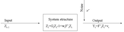
Fig. 2. Stochastic representation of input-output transformation model.

3 State-space model formulation

Clearly, there is a strict analogy between space and time, at least in the case of one-dimensional space. Hence, under the hypothesis of isotropy, analytical methods are to a broad extent equivalent. Typically, time series analysis allows us to analyse spatial structure in terms of autocorrelation func-tions and generalisation of state-space models. For this par-ticular method of regression in the time and space domain, unlike the methods of kriging and cokriging (Vieira et al., 1983) the assumption of stationarity of observations is not required. The state-space method (Kalman, 1960) is partic-ularly interesting when the phenomenon in question satis-fies certain systems of differential equations. The method has been used in economics (Shumway and Stoffer, 2000) and has yielded good results in agronomic and soil science (Vieira et al., 1983; Morkoc et al., 1985; Wendroth et al., 1992; Wu et al., 1997; Cassel et al., 2000; Poulsen et al., 2003; Nielsen and Wendroth, 2003)

Let us use Y(x),x=xo+1, ..., xo+n,to indicate the values assumed bynobservations made for a certain soil parame-terY along a given transect (below we shall use the simpler notationYt, t= 1, 2, ...,n). A state-space model consists,

in the formulation most useful for our purposes (for details and generalisations see Anderson and Moore, 1979), of two equations:

Yt=F 0 tZt+vt

Zt=GtZt−1+wt

isotropic

⇒

Zt=G1tZt−1+G2tZt+1+wt

anisotropic

t=1,2, ...n (1)

The first termed that of observations and the second that of transition, whereFt is a known vector (p, 1),Zt is a

vec-tor (p,1) of the system state, Gt,G1t, G2t are a set matrices

(p,p);vt∼N(0;σv2t)independent ofwt∼Np(0; P

wt). The

model (1) is wholly specified by the parameters (Ft, Git,σv2t, P

wt)and includes, as particular cases, other statistical

mod-els such as regression, ARIMA and SARMA modmod-els. Having set the initial values, we may obtain optimal fore-casts and estimates of the non-observable components by using the Kalman filter. At the same time, from many ob-servations made of soil physical and hydraulic properties, the latter may plausibly have been generated by stationary isotropic processes with parameters independent of the indi-vidual measuring points:

E(Yt)=µ; var(Yt)=σ2 cov(Yt,Yt±h)=c(h).

Hence we may consider the case in which the equations in (1) are reduced to simple ARMA and SARMA models. The importance of being able to make the double representation (state-space and SARMA or ARMA) lies in the fact that ARMA and SARMA models are easy to identify and esti-mate, while state-space models allow a more straightforward, immediate interpretation of the phenomena to which they are applied. Indeed, from (1) it follows thatYt may be

inter-preted as the result of signal F0_tZt which is overlaid by a

random errorvt. Evolution of many physical phenomena can

be well represented with a logical scheme like that reported in Fig. 2.

The system structure is usually very straightforward and can be approximated, in the isotropic case, by an AR(1), given by:

Zt=φZt−1+wt

or, in the anisotropic case, a SAR(1) given by: Zt=c0+φ1Zt−1+φ2Zt+1+wt

Note that, if it isφ1=φ2 then the SAR(1) model may be replaced by the simpler AR(1) model.

Moreover, if we assumep=1,F_t=1,Gt=φthen we

ob-tain more simply:

Yt=Zt+vt Zt=φZt−1+wt

⇔

(−φ B)Yt=(−α B)et

(1−φ B)Zt=wt , t

=1,2,...,n (2)

whereBis the backshift autoregressive operator,φi> αiand etsuch thatet−α1et−1−α2et+1=v−φ1vt−1−φ2vt+1+wt.

Thus both the equation of the observations and that of tran-sition (i.e. the signal) are reduced to simple ARMA models and especially to an ARMA (1,1) forYt and an AR(1) for

Zt.

Besides, as is widely acknowledged in soil physics, be-tween the many parameters there may well be functional re-lations such that what applies to the univariate cases can be extended to the simultaneous analysis in whichYt is anr

-dimensional vector. Under isotropic hypothesis, a particular generalisation of (1) to the case r=2 imply the following model:

Yt=FtZt+vt

Zt=GtZt−1+wt

;t=1,2,...,n (3)

where Ft is the (2, p) observation matrix which expresses

the pattern which converts the unobserved stochastic (p, 1) vectorZt into the (2, 1) vector observed seriesYt, and Gt a

(p,p) matrix of state-space coefficients or transition matrix indicating the measure of spatial regression

vt∼N2 0; X

vt !

independent of

wt∼Np 0; X

wt !

2458 A. Comegna et al.: State-space approach to evaluate spatial variability

Table 1. Descriptive indices of the spatial series observed along the transect at 0.3 m depth of soil profile.

Min Max Mean SD Skew Kurt CV

θ3(−) 0.307 0.383 0.341 0.019 0.217 −0.675 0.056

θ6(−) 0.257 0.330 0.287 0.018 4.462 −0.505 0.062

θ11(−) 0.205 0.283 0.239 0.016 0.256 −0.353 0.068

θ100(−) 0.236 0.300 0.257 0.015 0.655 −0.233 0.057

h3(cm) 58.0 103.1 83.2 10.4 −0.411 −0.217 0.125

h6(cm) 113.1 180.9 147.3 16.4 0.141 −0.700 0.111

h11(cm) 189.7 305.2 244.9 27.8 0.108 −0.670 0.113

Min = minimum value; Max = maximum value; SD = standard deviation: Skew = skewness; Kurt = kurtosis; CV = coefficient of variation.

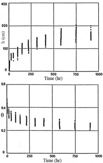
Fig. 3. Soil water tension (h) and volumetric water content (θas a function of time at the 0.3 m depth for all redistribution times during the drainage period.

In the particular case ofp=2, Ft= I with I the identical

ma-trix and Gt=8, we have the equivalent bivariate model:

Yt=Zt+vt Zt=8Zt−1+wt

⇔

(I−8B)Yt=(I−2B) et

(I−8B)Zt=wt t

=1,2,...,n

where et∼WN(0;6e)is independent of wt∼WN(0;6w)and

8are 2(2, 2) matrices of unknown parameters to be esti-mated.

4 Application in the univariate case

In this section we will analyze individually the two param-eters which characterize the soil water status in terms ofθ

andh measured at 0.3 m depth, along the N–S line of the plot so as to highlight their intrinsic structure linked to re-gional variability and, for 3 of the 12 measuring sampling times (the 3rd, 6th and 11th carried out 48, 168 and 768 h respectively from the start of the drainage), the variations oc-curring in time (the parameters concerned are indicated byθi

andhi).

The data were first elaborated using classical statistical techniques, hypothesizing that the parameters vary in an es-sentially random manner. From this point of view, the main statistical indices (min. value, max. value, mean, standard deviation, skewness, kurtosis, coefficient of variation) of the above parameters are reported in Table 1.

From Table 1 we may deduce, for all the measuring times considered, an increase in the standard deviation (SD) with its mean for parameter h, whereas the SD ofθis practically constant. We also note that the coefficient of variation (CV) ofhis almost twice that ofθ. Concluding, the two processes describingh andθ are, in time, both non-stationary on the mean, whileh is also non-stationary in variance. Figure 3 illustrates the above points: it reports the 50 observations of

θandhfor 10 of the 12 sampling times (from the 2nd to the 11th). This all agrees with the theoretical results obtained by Yeh et al. (1985), which predicted such behaviour on the basis of the stochastic analysis of unsaturated flow through heterogeneous media.

In the context of stochastic analysis it is essential to verify, for the parameters considered, the existence of a correlation structure.

A. Comegna et al.: State-space approach to evaluate spatial variability 2459

.26 .28 .30 .32 .34 .36 .38

.28 .30 .32 .34 .36 .38

f_2

f_

3

.30 .32 .34 .36 .38 .40 .42

.34 .36 .38 .40 .42 .44 .46

f_2

f_

3

a

b .26

.28 .30 .32 .34 .36

.28 .30 .32 .34 .36 .38

f_2

f_

3

.30 .32 .34 .36 .38 .40 .42

.34 .36 .38 .40 .42 .44 .46

f_2

f_

3

a

b

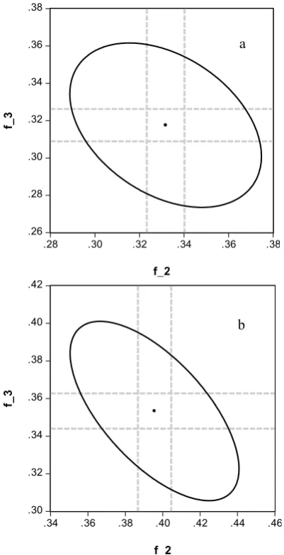
Fig. 4. 95% confidence region ofφ1andφ2parameters for (a)θ

and (b)hserie.

in terms of simplicity and interpretability, both because of the limited number of parameters and goodness of fit of the data, was SAR(1) model where the unknown parameters to be estimated areφ1andφ2. The above criteria of choice was followed for all models subsequently used. It should be noted that ifφ1andφ2are substantially equal thanθ3and h3are to be considered isotropic, conversely anisotropy may be taken into account.

The iterative least-squares method estimate of the model parameters in question, provided the results reported in Ta-ble 2 where standard deviations are in brackets. Having sup-posed that the phenomenon is isotropic and therefore invert-ible in space, the estimated φ1 andφ2values are expected to be equal. In particular, in our case, we may observe that

φ1=φ2. If the estimates are analyzed in greater detail, in the Fig. 4a, b it may be noted that the parameters in question are statistically identical. Then the model reported in (1) was

Table 2. Parameter estimates and comparison of SAR(1) model for the series examined and goodness of fit indexR2; in parenthesis the standard deviation of the estimates.

θ3 h3

c0 0.0858 29688.27

(0.0418) (12629)

φ1 0.3950 0.331

(0.1409) (0.1341)

φ2 0.3530 0.317

(0.1488) (0.1374)

σw 0.01435 8935.8

R2 0.4568 0.2907

Table 3. Parameter estimates of the ARMA(1,1) model, forθ3,h3,

θ100and goodness of fitR2. In parenthesis the standard deviations

of the estimated parameters.

φ α σˆl R2

θ₃ 0.94 (0.075) 0.51 (0.12) 0.0136 0.501

h3 0.91 (0.07) 0.63 (0.14) 8.729 0.300

θ100 0.77 (0.10) 0.21 (0.10) 0.0110 0.392

applied, only to three series of data obtained along the tran-sect. The series concerns, in particular, values of soil water contentθand tensionhobtained 48 h from the beginning of the drainage. Furthermore the analysis will be extended to a section of the soil moisture retention curveθ(h) constructed forh=100 cm, subsequently indicated asθ100.

More significantly, the essential characters assumed in the space from the distribution of the parameters in question may be deduced from the transects of Fig. 5, which report the relative values in the 50 observation points.

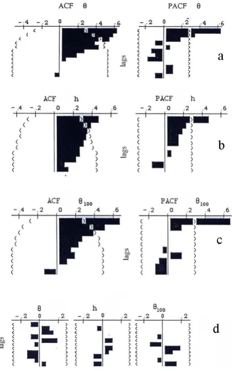
To identify the ARMA models to be adapted to the above three series, we estimated the autocorrelation (ACF) and par-tial autocorrelation (PACF) function. As transpires from Fig. 6a, b, c, the three series can be well represented by an ARMA (1,1) model.

Anyway analysis of ACF residuals (Fig. 6d) shows clearly that no structure whatever is present in the series of noises, which is further confirmation of the good fit of the model used to represent the examined parameters.

2460 A. Comegna et al.: State-space approach to evaluate spatial variability

0.00 0.05 0.10 0.15 0.20 0.25 0.30 0.35 0.40 0.45

0 10 20 30 40 50

Distance along the transect (m)

θ

a

0 20 40 60 80 100

0 10 20 30 40 50

Distance along the transect (m)

h (cm

)

b

0.00 0.05 0.10 0.15 0.20 0.25 0.30 0.35 0.40

0 10 20 30 40 50

Distance along the transect (m) θ100

c 0.00

0.05 0.10 0.15 0.20 0.25 0.30 0.35 0.40 0.45

0 10 20 30 40 50

Distance along the transect (m)

θ

a

0 20 40 60 80 100

0 10 20 30 40 50

Distance along the transect (m)

h (cm

)

b

0.00 0.05 0.10 0.15 0.20 0.25 0.30 0.35 0.40

0 10 20 30 40 50

Distance along the transect (m) θ100

c 0.00

0.05 0.10 0.15 0.20 0.25 0.30 0.35 0.40 0.45

0 10 20 30 40 50

Distance along the transect (m)

θ

a

0 20 40 60 80 100

0 10 20 30 40 50

Distance along the transect (m)

h (cm

)

b

0.00 0.05 0.10 0.15 0.20 0.25 0.30 0.35 0.40

0 10 20 30 40 50

Distance along the transect (m) θ100

c

Fig. 5. Measured values of: (a) soil water contentθ3, (b) soil water

tensionh3and (c) soil water contentθ100, ath=100 cm.

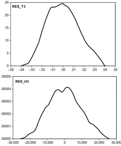
both ARMA(1,1) models end the null hypothesis (normality distribution) is accepted. The kernel estimate residuals dis-tributions are reported in Fig. 7.

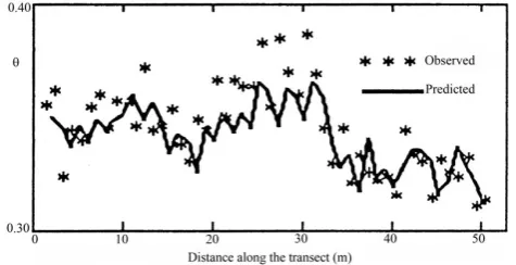
The estimated model was then used to obtain optimal pre-dictions along the transect. Figure 8a, b reports the observed data, a signal estimate and the relative noise for seriesθ3and

h3. The graphs for the other series were similar, with anal-ogous signal in the general pattern, not reported here for the sake of brevity, confirming that the spatial structure of soil hydraulic parameters is a characteristic of the porous medium in question.

Fig. 6. Estimated ACF and PACF functions with approximate 95% confidence bond, for: (a) soil water contentθ3, (b) soil water

ten-sionh3, (c) water contentθ100, ath=100 cm and (d) noise in model

1 forθ3,h3,θ100.

5 Application in the bivariate case

Consistent with the aim of simultaneously analysing param-etersθ andhas a bivariate dynamic system and modelling statistically the intrinsic variability, in this section we seek to ascertain once again the suitability of the multivariate ap-proach based on the use of state-space models. Preliminary qualitative assessment regarding the nature of the functional relationship betweenθ andh may be inferred from inspec-tion of figure 9 which reports all theθandhvalues measured contemporaneously for each of the 50 sites and for 10 of the 12 measuring times.

A. Comegna et al.: State-space approach to evaluate spatial variability 2461

0 5 10 15 20 25

-.05 -.04 -.03 -.02 -.01 .00 .01 .02 .03 .04 .05

RES_T3

(left)

.00000 .00001 .00002 .00003 .00004 .00005

-30,000 -20,000 -10,000 0 10,000 20,000 30,000

RES_H3

(right) 0

5 10 15 20

-.05 -.04 -.03 -.02 -.01 .00 .01 .02 .03 .04 .05

(left)

.00000 .00001 .00002 .00003 .00004 .00005

-30,000 -20,000 -10,000 0 10,000 20,000 30,000

RES_H3

(right)

Fig. 7. Kernel density residual estimation from model ARMA(1, 1) for parameterθ3(up) andh3(below).

with a curve to which the analytical expression proposed by van Genuchten (1980) was assigned:

θ (h)=θr+

θs−θr

1+ |αh|nm h <0 (4)

θ (h)=θs h≥0 (5)

whereθsandθr denote the saturated and residual water

con-tent respectively. The constantsα,mandnare shape param-eters andm=1−1

n.

The estimate of parameter (α,n)in model and the good-ness index of fitR2, obtained by the least squares method, led to the following results: θr= 0, α= 0.01, n= 1.46 and R2= 0.90.

The problem that arises at this point is to ascertain whether the bivariate model is compatible with the results obtained for the individual variablesθ andh. In this respect, it can be easily verified that a bivariate ARMA(1,1) means that the single components are univariate ARMA(2,2) in contrast to ARMA(1,1) models that are adaptable toθ andh. Admit-tedly, the situations between the elements8and2may co-incide, hence ARMA(2,2) are simplified into ARMA(1,1). However, the constraints to be met are such as to rule out that this may in practice occur. On the other hand, if in (3) we havevt= 0, thenYt coincides withZt and this has two

implications: (a) it can no longer be supposed thatθandh

are broken down simultaneously into a signal and an error

-.03 -.02 -.01 .00 .01 .02 .03

.30 .32 .34 .36 .38 .40

5 10 15 20 25 30 35 40 45

Residual Actual Fitted

Distance along the transect (m) theta

3 a

θ3

b -.03 -.02 -.01 .00 .01 .02 .03

.30 .32 .34 .36 .38 .40

5 10 15 20 25 30 35 40 45

Residual Actual Fitted

Distance along the transect (m) theta

3 a

θ3

b

Fig. 8. Values of (a)θ3and (b)h3, observed, fitted and predicted

with ARMA(1,1) model.

0.0 0.1 0.2 0.3 0.4 0.5 0.6 0.7

0 100 200 300 400 500 600 700

h (cm)

θ

Fig. 9. Scatter ofθ(h) values observed in the field along the transect at 0.3 m depth of soil profile.

(this does not exclude the decomposition of single compo-nents); (b) the ARMA structure ofYt is simplified into the

bivariate AR(1) model:

(I−8B)Yt=wt (6)

2462 A. Comegna et al.: State-space approach to evaluate spatial variability

Fig. 10. Schematic representation of cross correlation matrices of estimated residues: () auto-cross correlations non significantly different from zero, ( – ) auto-cross correlation significantly greater than zero.

ARMA(1,1) obtained empirically for the components, but in this case the coincidental conditions such that an ARMA(2,1) is reduced to an ARMA(1,1), are not very constraining. Hence it is plausible that the bivariate model forY_t is type (6). Moreover, it is easy to prove that model (6), through orthogonalization of6w, may equally be represented by the

following:

θt=c1+β1ht+β2θt−1+β3ht−1+at

ht=c2+δ1θt+δ2ht−1+δ3θt−1+bt (7)

which expresses the simultaneous functional relation be-tweenθandh. Note that in Eq. (3),atandbtare white noises

independent among them and respectively with ht and θt.

Moreover, the proof is straightforward that if8= Diag{φ11,

φ22}then we also obtainβ2=φ11and δ2=φ22.

The estimates of the bivariate AR(1) and the relative cor-relation matrix of the residuals are:

ˆ

8 =



 0.60

(0.12)

0 0 0.48

(0.13)



; R=

1 −0.38

−0.38 1

while the first 10 auto cross-correlations matrices of the es-timated residuals, for exploratory purposes are reported syn-thetically in Fig. 10.

From these it emerges that the bivariate AR(1) model fits the two phenomena well and highlights the existence of si-multaneous causal relations, as was to be expected, between

θandh. Estimation with the least squares of model (3) sup-plied the following results (in brackets the mean square de-viations of the estimates):

 

 ˆ θt=0.13

(2.8)

−0.00061 (−2.71) ht

+0.68 (5.94)θt−1

+0.00036 (1.55) ht−1

;R2=0.48

ˆ

ht=54.5

(1.82) −231.1

(−2.73)θt +0.49

(3.9)ht−1 +193.88

(2.18) θt−1

;R2=0.33 (8)

As may be noted, this yieldsβˆ2≈ ˆφ11 andδˆ2≈ ˆφ22 which may be considered further confirmation of the goodness of the statistical model used to interpret and describe the two parametersθt andhtand the relations between them. In this

respect, in Fig. 11 we report theθtvalues observed and those

estimated with the first of (4). The expression manages to capture the phenomenon’s general trend. A similar relation-ship, albeit not presented, is obtained for the second of (4).

Fig. 11. Water contentθ3observed and estimated with the first of

Eq. (8).

6 Conclusions

The soil water status may be better defined stochastically rather than deterministically since it is not always possible to evaluate with precision the behaviour of parametersθand

h of the flow system at an assigned point in time. This is due both to intrinsic and extrinsic heterogeneities of natural porous media, and to field crop root water uptake as well as natural contributory factors which are essentially stochastic. The experiment carried out on a field plot on a Vesuvian volcanic soil, with regard to its water status, showed thatθ

andhare essentially multi-dimensional processes when ob-served in space and time. The isotropic nature of the phe-nomena are firstly empirical verified and then the space cor-relation structures were analyzed using state-space methods which allowed the setting-up of univariate models. The non-stationary nature of soil water tension, in mean and in vari-ance was then ascertained, whereas water content was locally stationary on mean and variance for the whole period of ob-servation. In any case, the signals in the observed series were fairly clear and marked even if influenced in complex manner by the water dynamics of the soil profile.

The deterministic relations between θ and h suggested the use of bivariate models which allowed for any simulta-neous isotropic relations existing between the two parame-ters in space. The theoretical potential and the practical im-plications of these results in the modelling of water trans-port processes in unsaturated heterogeneous porous media require further in-depth studies above all with regard to dif-ferent pedological contexts from those here analyzed. Since drainage is the predominant transport process in this simpli-fied hydrological experiment, it is reasonable to suppose that it depends upon the combined effect of soil conducting prop-erties within the entire soil profile.

Edited by: S. Grimaldi

References

Anderson, B. D. C. and Moore, J. B.: Optimal filtering, Englewood Cliffs, N. J., Prentice Hall, 1979.

Anderson, S. H. and Cassel, D. K.: Statistical and autoregressive analysis of soil properties of Portsmouth Sandy Loam, Soil Sci. Soc. Am. J., 50, 1096–1104, 1986.

Box, G. E. P. and Jenkins, G. M.: Time Series Analysis, Forecasting and Control, Holden Day, San Francisco, 1970.

Cassel, D. K., Wendroth, O., and Nielsen, D. R.: Assessing spatial variability in an agricultural experiment station field: opportu-nities arising from spatial dependence, Agron. J., 92, 706–714, 2000.

Feddes, R. A., Kebat, P., and Van Bakel, P. J. T.: Modelling soil wa-ter dynamics in the unsaturated zone, State of art, J. of Hydrol., 100(1/3), 69–111, 1998.

Freeze, R. A.: A stochastic conceptual analysis of one-dimensional groundwater flow in nonuniform heterogeneous media, Water Resour. Res., 11, 725–741, 1975.

Heuvelink G. B. M. and Webster, R.: Modeling soil variation: past, present and future, Geoderma, 100, 269–301, 2001.

Hillel, D.: Environmental Soil Physics, Academic Press, 1998. Kalman, R. E.: A new approach to linear filtering and predictions

problems. Transactions of ASMA, D. Jour. of Basic Enginering, 82, 35–45, 1960.

Matheron, G.: The theory of regionalized variables and its applica-tions, Ecole des Mines de Paris, Fontainbleau, 1971.

Morkoc, F., Biggar, J. W., Nielsen, D. R., and Rolston, D. E.: Anal-ysis of soil water content and temperature using state-space ap-proach, Soil Sci. Soc. Am. J., 49, 798–803, 1985.

Nielsen, D. R., Biggar, J. W., and Erh, K. J.: Spatial variability of field measured soil water properties, Hilgardia, 42, 215–259, 1973.

Nielsen, D. R. and Wendroth, O.: Spatial and temporal statistics, Series: Adv. Geoecol., Catena, 2003.

Poulsen, T. G, Moldrup, P., Wendroth O., and Nielsen D. R.: Es-timating saturated hydraulic conductivity and air permeability from soil physical properties using state-space analysis, Soil Sci., 168, 311–320, 2003.

Russo, D. and Bresler, E.: Soil hydraulic properties as stochastic process. 1. An analysis of field spatial variability, Soil Sci. Soc. Am. J., 45, 682–687, 1981.

Shumway, R. H. and Stoffer, D. S.: Time series analysis and its applications, Springer Verlag, New York, 2000.

Snedecor, G. W. and Cochran, W. G.: Statistical Methods, 7th edi-tion, Iowa State Universiry Press, Ames, Iowa, 1980.

van Genuchten, M. Th.: A closed form equation for predicting the hydraulic conductivity of unsaturated soils, Soil Sci. Soc. Am. J., 44, 892–898, 1980.

Vieira, S. R., Nielsen, D. R., and Biggar, J. W.: Spatial variability of field measured infiltration rate, Soil Sci. Soc. Am. J., 45, 1040– 1048, 1981.

Vieira, S. R., Hatfield, J. L., Nielsen, D. R., and Biggar, J. W.: Geostatistical theory and applications to variability of some agro-nomical properties, Hilgardia, 51, 1–72, 1983.

Vitale, C.: Considerazioni critiche sulla scomposizione dei modelli ARIMA, Rivista di Statistica Applicata, 13, 91–104, 1980. Yeh, T. C. J., Gelhar, L. W., and Gutjahr, A. L.: Stochastic

anal-ysis of unsaturated flow in heterogeneous soils. 2. Statistically anisotropic media, Water Resour. Res., 21, 457–464, 1985. Wendroth, O., Al-Omran, A. M., Kirda, C., Reichardt, K., and

Nielsen, D. R.: State-space approach to spatial variability of crop yield, Soil Sci. Soc. Am. J., 56, 801–807, 1992.

Wendroth, O., Koszinski, S., and Pena-Yewtukhiv, E.: Spatial as-sociation between soil hydraulic properties, soil texture and geo-electric resistivity. Vadose Zone J., 5, 341–355, 2006.