Full Length Research Article
HIGH
PERFORMANCE
SPEED
OF
THE
INDUCTION
MOTOR
DRIVES
BY
THE
PREDICTIVE
CONTROL
USING
SPACE
VECTOR
MODULATION
*Lakhdar Djaghdali, Belkacem
Sebti and Farid Naceri
Department of Electrical Engineering, University of Batna Street Chahid Med El Hadi boukhlouf, Batna 05000,
Algeria
ARTICLE INFO ABSTRACT
This paper investigates the application of the generalized predictive control (GPC), in order to control the speed of the induction motor. This application is based on four main ideas : reproducing decision basic mechanisms of human behaviour; the creation of an anticipatory effect by operation of the path to follow in the future; defining a numerical prediction model; minimization of a quadratic criterion with finite horizon and the principle of receding horizon. The results proved that the induction motor with the MPC speed controller has superior transient response, and good robustness in face of uncertainties including load disturbance. Moreover, accurate tracking performance has been achieved.
Copyright © 2015 Lakhdar Djaghdali et al.This is an open access article distributed under the Creative Commons Attribution License, which permits unrestricted use, distribution, and reproduction in any medium, provided the original work is properly cited.
INTRODUCTION
AC induction motors have been widely used in industrial applications such as machine tools, steel mills and paper machines owing to their good performance provided by their solid architecture, low moment of inertia, low ripple of torque and high starting torque. some control techniques have been developed to regulate these induction motors servo drives in
high-performance applications. One of the most popular technique is the indirect field oriented control method (Egiguren et al., 2008).
The field-oriented technique guarantees the decoupling of torque and flux control commands of the induction motor, so that the induction motor can be controlled linearly as a separated excited d.c. motor. However, the control performance of the resulting linear system is still influenced by uncertainties, which are usually composed of unpredictable parameter variations, external load disturbances, measurement noise and unmodelled and nonlinear dynamics. therefore, many studies have been made on the motor drives in order to preserve the performance under these parameter variations and external load disturbances, such as nonlinear
control, optimal control, variable structure system control, adaptive control, neural control and predictive control (Egiguren et al.,
2008 and Marino et al., 1998).
Since D. Clarke proposed in 1987 (Clarke et al., 1987) the generalized predictive control design principles, a lot of authors have
used this advanced technique in induction motors control. in the past decade, the generalized predictive control strategy has been focused on many studies and research for the control of the ac servo drive systems. The generalized predictive control lets to know the future sequence of the output and thus it is possible to calculate the optimal control signal for that output, when the reference is known a priori. In these sense, the system can react before the change has effectively been made, thus avoiding the
effects of delay in the process response, (Egiguren et al., 2008). Generally, for a greater number of the know future samples, the
obtained control signal is better that the contrary case, but with the inconvenient of greater computation requirements for the
controller, (Kennel et al., 2001).
*Corresponding author: Lakhdar Djaghdali
Department of Electrical Engineering, University of Batna Street Chahid Med El Hadi boukhlouf, Batna 05000, Algeria
ISSN: 2230-9926
International Journal of Development Research
Vol. 5, Issue, 06, pp. 4645-4654, June,2015International Journal of
DEVELOPMENT RESEARCH
Article History: Received 21st March, 2015
Received in revised form 30th April, 2015
Accepted 06th May, 2015
Published online 28th June, 2015 Key words:
Induction Motor, Predictive control,
Space vector modulation (SVM).
However the gpc has other issues. on the one hand, it has the added difficulty of the existence of constraints, that is, the study of the control system taking account the limitations of the real system like saturation values, frequency and time limits, etc,
(Egiguren et al., 2008 and Rodríguez and Dumur, 2005). On the other hand, it has to be dealt with the presence of external
disturbances (Camacho and Bordons, 2004) (known and unknown) and measurement of noise. Other important issue is the
robustness of the gpc controller, (Egiguren et al., 2008 and Rodríguez and Dumur, 2005).
In this paper, we present some brief philosophy of the principle and the interests of predictive control, we applied this command on the induction machine for speed control (fig. 3), where the torque and flux are regulated by pi controller (Belkacem, 2011 and Lai and Chen, 2001). The control voltages can be generated by pi and imposed by SVM technique (Zhou and Wang, 2002). In addition, the estimate of the torque and flux are based on the model of the machine voltage. The results of simulation show high dynamic performance.
MODEL OF THE MACHINE FOR THE CONTROL
Among the various types of models used to represent the induction machine, there is one that uses each of the stator currents, stator flux, and speed as state variables and voltages (Vsd, Vsq) as control variables. This model is presented in reference (d, q), related to the rotating field. This model is expressed by the following system of equations (Carloss, 2000 and Grellet and Clerc, 2000):
⎩
⎪
⎪
⎨
⎪
⎪
⎧
=
.
+
−
.
=
.
+
+
.
= 0 =
.
+
− (
−
Ω
).
= 0 =
.
+
+ (
−
Ω
).
(1)
In addition, the components of the stator and rotor flux are expressed by:
⎩
⎨
⎧
=
=
.
.
+
+
.
.
=
.
+
.
=
.
+
.
(2)
Moreover, the mechanical equation of the machine is given by:
Ω
+
Ω
=
−
(3)The electromagnetic torque equation can be expressed in terms of stator currents and stator flux as follows:
= . (
.
−
.
)
(4)Where :(
,
) ;(
,
) ;(
,
); (
,
) are currents, voltages, and stator and rotor flux axis d-q.
(
,
) : stator and rotor resistance.
(
,
) : stator and rotor
Cyclic
Inductance.
(L
m, p): mutual Inductance and Number of pole pairs.
(
,
Ω
): Stator pulsation and mechanical rotor speed.
THE PHILOSOPHY OF THE PREDICTIVE CONTROL
Fig.1. Time Evolution of the Finite Horizon Prediction
THE PRINCIPLE AND GENERAL STRATEGY OF PREDICTIVE CONTROL
The basic principle of predictive control is taken into account, at the current time of the future behavior, through explicit use of a
numerical model of the system in order to predict the output on a finite horizon in the future, (Ahmed A. Zaki Diab et al., 2013).
One of the advantages of predictive methods lies in the fact that for a pre-calculated set on a horizon, it is possible to exploit the information of predefined trajectories located in the future, given that the aim is to match the output of system with this set on a finite horizon.
In general, the predictive control law is obtained from the following methodology:
Predict future process outputs the prediction horizon defined by using the prediction model. These outputs are dependent on the output values of the input process known to control up to time t (Camacho and Bordons, 2003). Determine the sequence of control
signal, by minimizing a performance criterion to conduct the process output to an output reference (Garcia et al., 1989). Usually
the performance criterion to be minimized is a compromise between a quadratic function of the error between the predicted output and the desired future, and the cost of control effort. Moreover, the minimization of such a function can be subject to state constraints and more generally to constraints on the order. The control signal u (t) is sent to the process while the other control signals are ignored at time t +1, we acquire the actual output y (t +1) and again in the first (Papafotiou and Kley, 2009 and Camacho and Bordons, 2003).
INTERESTS OF THE PREDICTIVE CONTROL
Most industrial regulations are often made with analog PID controllers with remarkable efficiency and price/performance ratio with which it is difficult to compete. However, this type of controller does not cover all the needs and the performance suffers in a range of applications which we quote:
Difficult Process, especially nonlinear, unsteady, high pure delay and also multivariate (Karamanakos et al., 2014). When
performance is tensioned by the user, including: high attenuation of disturbances, following error zero tracking, minimum response time, which leads to function under constraints that affect on the control variables, and even the internal variables of the
process (Camacho and Bordons, 2003 and Karamanakos et al., 2014). Wealth of predictive control arises from the fact that it is
not only capable of controlling simple processes of the first and second order, but also complex processes, including processes with time delay long enough, unstable loop process opened without the designer takes special precautions too. During the last
years, different predictive controller structures have been developed (Garcia et al., 1989), including the generalized predictive
control (GPC).
GENERALIZED PREDICTIVE CONTROL
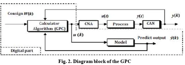
The generalized predictive control (GPC) of Clarke (Papafotiou and Kley, 2009), is considered as the most popular method of prediction, especially for industrial processes. This resolution is not repeated each time there is an optimal control problem: "how to get from the current state to a goal of optimally satisfying constraints" (Rawlings and Mayne, 2009). For this, you must know at each iteration the system state using a numerical tool. Temporal representation of generalized predictive control is given by (Fig.2), where there are controls u(k) applied to the system for rallying around the set point w (k). Numerical model is obtained by a discretization of the continuous transfer function of the model which is used to calculate the predicted output of a
finite horizon.
Fig. 2. Diagram block of the GPC
FORMULATION OF THE MODEL
All predictive control algorithms differ from each other by the model used to represent the process and the cost function to be minimized. The process model can take different representations (transfer function by state variables, impulse response...), for our formulation, the model is represented as a transfer function.
CRITERION OPTIMIZATION
We must find the future control sequence to apply the system to reach the desired set point by following the reference trajectory. To do this, we just minimize a cost function which differs according to the methods. But generally this function contains the squared errors between the reference trajectory, the predictions of the prediction horizon and the variation of the control (Boucher and Dumur, 1996). This cost function is as follows:
= ∑ [ ( + ) − ( + )] + ∑ Δ ( + − 1) (5)
With:
w (t + j): Set point applied at time (t + j).
y
ˆ
(
t
j
): Output predicted time (t + j).
Δu(t + j-1): Increment of control at the moment
(t + j-1).
N
1: Minimum prediction horizon on the output.
N
2: maximum Prediction Horizon on the output with N
2≥ N
1.
N
u: prediction Horizon on the order.
λ: Weighting factor on the order.
T
s: The period of sampling.
The criteria expression call for several comments:
When there are actually values of the set point in the future, all of these informations are used between horizons of N1 and N2 so
as to converge the predicted output to this set point. There is the incremental aspect of the system by considering ∆u in the criteria. The coefficient λ is used to give more or less weight to the control relative to the output, so as to ensure the
convergence when the starting system is a risk of instability (Qin and Badgwell, 2003).
CHOICE OF THE PARAMETERS OF CONTROL
The definition of the quadratic criterion (l’eq-5) showed that the user must set four parameters. The choice of parameters is difficult because there is no empirical relationship to relate these parameters to conventional measures in automatically.
N1: minimum horizon of prediction is the pure delay system, if the delay is known or we should initialize to 1.
N2: maximum horizon is chosen so that the product N2Ts is limited by the value of the desired response time. Indeed increase
beyond the prediction of the response time provides no additional information. In addition, the more N2 is larger, the system is stable and slow.
Nu: horizon of control, we should choose equal to 1 and not exceeding the value of two.
λ: weighting factor of the order, this is the most complicated to set parameter since it influences the stability of the closed loop
REGULATING THE SPEED OF THE INDUCTION MACHINE BY PREDICTIVE CONTROL
We will regulate the speed of the induction machine by the laws of predictive control (Fig. 3). This figure comprises two loops one with two internal PI controllers is used to control the torque and flux and the other external to regulate the speed based on predictive control laws presented above. The transfer function of the torque-speed end of the mechanical equation can be represented in the ongoing plan by the following transfer:
f
js
s
T
s
e
1
)
(
)
(
* [image:5.595.129.458.145.344.2]Fig. 3. Block diagram the speed control of the IM by the predictive control
SPACE VECTOR PULSE WIDTH MODULATION
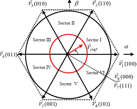
The voltage vectors, produced by a 3-phase PWM inverter, divide the space vector plane into six sectors as shown in (Fig. 4).
Fig. 4. The diagram of voltage space vectors
In every sector, the voltage vector is arbitrary synthesized by basic space voltage vector of the two sides of one sector
and zero vectors. For example, in the first sector, Vs ref is a synthesized voltage, space vector and its equation is given
by (Zhou and Wang, 2002).
(6)
Sector I Sector II
II2 Sector III
Sector IV
Sector V
Sector VI
1(100)
V
sref
V
0(000)
V
7(111)
V
6(101)
V
5(001)
V
4(011)
V
3(010)
V V2(110)
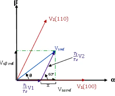
[image:5.595.201.429.429.611.2]Where, T0, T1 and T2 is the work time of bas
Fig.
The determination of the amount of times T1
=
| | +
=
| | sin( )
=
( )
The rest of the period is applying the null-vect implementation can all be related to the Follo
=
√2
=
√6
+ √2
=
−√6
+ √2
The implementation of the duration sector boundary vectors are tabulated as follows:
Sector
T
The third step is to compute the duty cycles h
T
aon=
T
bon= T
aon +T
con= T
bon+
sic space voltage vectors V0, V1 and V2 respectively
ig. 5. Projection of the reference voltage vector
and T2 given by mere projections is:
=
√6
− √2
=
√ector. For every sector, switching duration is calculate owing variables:
(10)
The implementation of the duration sector boundary vectors are tabulated as follows:
Table 1. Durations of the sector boundary vectors
Sector
1
2
3
4
5
6
T
I-Z
Y
X
Z
-Y
-X
T
I+1X
Z
-Y
-X
-Z
Y
have three necessary times:
(11)
y.
(9)
ted. Amount of times the vector
[image:6.595.193.393.77.244.2]
Table 2. Assigned duty cycles to the PWM outputs
Sector
1
2
3
4
5
6
S
aT
aonT
bonT
conT
conT
bonT
aonS
bT
bonT
aonT
aonT
bonT
conT
conS
cT
conT
conT
bonT
aonT
aonT
bonRESULTS OF SIMULATION
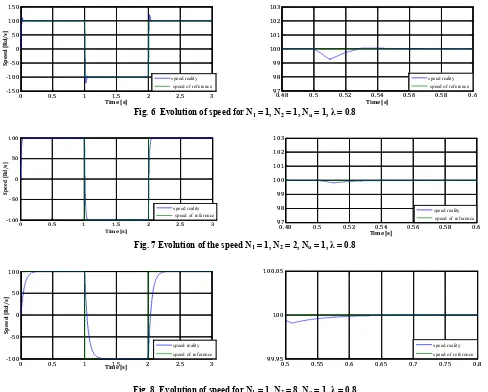
In the absence of general analytical rules leading to the choice of the synthesis parameters of a predictive control based on the type of process and required performance, the implementation practice always requires several simulation tests to finally arrive at an optimal choice. To test the effectiveness of the control strategy is going to make the choice to optimize the controller parameters by changing the parameters each one and see their effect on the performance of control, leading to a better choice of (speed, response time, overshoot, stability etc ....). To illustrate the performance of the predictive control applied to the speed control, the machine was simulated with a reference speed of 100 rd/s vacuum and then applying a nominal load of 20 Nm at t = 0.5 s to t = 1 s, then the motor is subjected to a target change speed 100 rd/s to -100rd/s.
a. INFLUENCE THE HORIZON OF PREDICTION N2
N2 is varied to see its effect on performance. The following figures show the evolution of the output (speed of induction machine)
for different values of N2.
Fig. 6 Evolution of speed for N1 = 1, N2 = 1, Nu = 1, λ = 0.8
[image:7.595.51.539.341.733.2]Fig. 7 Evolution of the speed N1 = 1, N2 = 2, Nu = 1, λ = 0.8
Fig. 8 Evolution of speed for N1 = 1, N2 = 8, Nu = 1, λ = 0.8
0 0.5 1 1.5 2 2.5 3
-150 -100 -50 0 50 100 150 Time [s] Sp e e d [R d /s ]
The answer of the cosigne crenel speed (100 to -100 rd/s)
speed reality speed of reference
0.48 0.5 0.52 0.54 0.56 0.58 0.6
97 98 99 100 101 102 103 Time [s] speed reality speed of reference
0 0.5 1 1.5 2 2.5 3
-100 -50 0 50 100 Time [s] Spe ed [ Rd /s ] speed reality
speed of reference
0.48 0.5 0.52 0.54 0.56 0.58 0.6
97 98 99 100 101 102 103 Time [s] speed reality speed of reference
0 0.5 1 1.5 2 2.5 3 -100 -50 0 50 100 Time [s] S p e e d [ R d /s ] speed reality
speed of reference
0.5 0.55 0.6 0.65 0.7 0.75 0.8 99.95
100 100.05
speed reality
speed of reference
DISCUSSION OF THE RESULTS
It is remarkable that a significant increase in the prediction horizon (N2) results in a slow response in the system while a too strong
decrease results in a large overshoot of the set point. Time mounted increases with a positive variation of N2 and decreases with a
negative variation of N2.
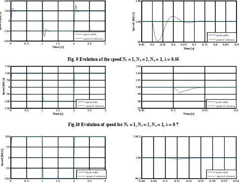
b. INFLUENCE THE WEIGHTING COEFFICIENT λ
λ is varied to see its effect on performance. The following figures show the evolution of the output (speed of the machine) for deferent values of λ.
[image:8.595.46.530.203.571.2]Fig. 9 Evolution of the speed N1 = 1, N2 = 2, Nu = 1, λ = 0.55
Fig.10 Evolution of speed for N1 = 1, N2 = 2, Nu = 1, λ = 0.7
Fig.11 Evolution of speed for N1 = 1, N2 = 2, Nu = 1, λ = 0.9
DISCUSSION OF THE RESULTS
From the system response for deferent values of λ, we see an increase in weighting on the control (λ) results in a decrease in the response time of the system, resulting in a decrease exceeded set point.
CONCLUSION
In this article we have given a brief philosophy and the principle of predictive control. This command is a combination between the prediction of future behavior of the process and control feedback. We applied this command to the speed control of the
0 0.5 1 1.5 2 2.5 3 -200 -100 0 100 200 Time [s] Sp e e d [R d /s ] speed reality
speed of reference
0.45 0.5 0.55 0.6 0.65 0.7 0.75 0.8 0.85 0.9 95 100 105 Time [s] S p e e d [R d /s ] speed reality
speed of reference
0 0.5 1 1.5 2 2.5 3
-150 -100 -50 0 50 100 150 Sp e e d [ R d /s ] Time [s] speed reality speed of reference
0.45 0.5 0.55 0.6
97 98 99 100 101 102 103 Time [s] speed reality speed of reference
0 0.5 1 1.5 2 2.5 3
-100 -50 0 50 100 Time [s] Sp e e d [R d /s ] speed reality speed of reference
0.48 0.49 0.5 0.51 0.52 0.53 0.54 0.55 0.56
99.5 100 100.5
Time [s]
We noted that the major drawback of predictive control is that the performance is greatly influenced by the choice of the
synthesis parameters N1, N2, Nu, and λ therefore, a judicious choice of these parameters is necessary before the
implementation of the simulation algorithm, to meet the desired performance.
CHARACTERISTICS OF THE MACHINE USED FOR SIMULATION
parameter symbol Value
Number of pole pairs p 2
Power Pu 3 KW
Line voltage Un 380V
Line urrent In 6.3A
Nominal frequency f 50Hz
Mechanical rotor speed Nn 1430 tr/mn
Electromagnetic torque Te 20Nm
Stator Resistance Rs 3.36 Ω
Rotor Resistance Rr 1.09 Ω
Stator cyclic inductance Ls 0.256H
Mutual cyclic Inductance Lm 0.236H
Rotor cyclic inductance Lr 0.256H
Rotor inertia j 4,5. 10 Kg. m2
Viscosity coefficient f 6,32.10 N.m.sec.
REFERENCES
Ahmed A. Zaki Diab, Denis A. Kotin and Vladimir V. Pankratov, 2013. “Speed Control of Sensorless Induction Motor Drive Based On Model Predictive Control”. XIV international conference on micro/nanotechnologies and electron devices, 978-1-4799-0762-5/13/$31.00 © 2013 IEEE
Belkacem, S. 2011. “High Performance Direct Torque Control of Induction Motor Drive Using SVPWM”. 11th International Conference on Control, Automation and Systems Oct. 26-29, KINTEX, Gyeonggi-do, Korea.
Boucher, P. a nd D. Dumur, 1996. “The Predictive Control” collection methods and practices of the engineer, central school of Lille.
Camacho, E. F. and C. Bordons, 2004. “Control Predictivo: pasado, presente y futuro”. ETSI, Universidad de Sevilla, CEA- IFAC, Sevilla, Spain.
Camacho, E.F. and C. Bordons, 2003. “Model Predictive Control”, Springer-Verlag London, 2eme edition. Carloss, C. 2000. “Modeling Vectorial Control et DTC”. Edition Hermes Sciences Europe.
Clarke, D. W., C. Mohtadi and P. S. Tuffs, 1987. “Generalized Predictive Control -Part I. The Basic Algorithm”, Automatica, Vol. 23, NO. 2, pp. 137-148.
Clarke, D. W., C. Mohtadi and P. S. Tuffs, 1987. “Generalized Predictive Control – Part II. Extensions and Interpretations”, Automatica, Vol. 23, No. 2, pp. 149-160.
Egiguren, P., O. Caramazana§, A. Hernández and I. Garrido Hernández, 2008. “SVPWM Linear Generalized Predictive Control of Induction Motor Drives”, university of the Basque Country. Avda de Otaola 29, 20600. Eibar (Spain) pp. 588-593. IEEE. Garcia, C. E., D. M. Prett and M. Morari, 1989. “Model Predictive Control: Theory and Practice – A Survey”. Automatica,
25(3):335–348.
Grellet, G. a nd G. Clerc, 2000. “Actionneurs Electriques, Principe, Modèles, Commande”. Collection Electrotechnique. Edition Eyrolles.
Karamanakos, P., P. Stolze, R. M. Kennel, S. Manias and H. Mouton, 2014. “Variable Switching Point Predictive Torque Control of Induction Machines”. IEEE journal of emerging and selected topics in power electronics, vol. 2, no. 2.
Kennel, R., Linder, A. and Linke, M. 2 001. “Generalized Predictive Control (GPC)-Ready for use in drive applications”. University of Wupepertal, Germany.
Lai, Y. S. a n d J. H. Chen, 2001. “A New Approach to Direct Torque Control of Induction Motor Drives for Constant Inverter Switching Frequency and Torque Ripple Reduction”, IEEE Trans. Energy Conv. 16.
Marino, R., S. Peresada and P. Tomei, 1998. “Adaptive Output Feedback Control of Current-Fed Induction Motors with Uncertain Rotor Resistance and Load Torque.”, Automatica, 34, pp. 617-624.
Papafotiou, G., J. Kley, K. G. Papadopoulos, P. Bohren and M. Morari, 2009. “Model predictive direct torque control - part II: Implementation and experimental evaluation”. IEEE Trans. Ind. Electron., 56(6):1906–1915.
Qin S. J. and T. A. Badgwell, 2003. “A Survey of Industrial Model Predictive Control Technology”. Control Engineering Practice, 11(7):733–764.
Rawlings, J. B. and D. Q. Mayne, 2009. “Model predictive control: Theory and design”. Nob Hill Publ.
Rodríguez, P. and Dumur, D. 2005. “Generalized Predictive Control Robustification Under Frecuency and Time Domain Constraints”, IEEE Transactions on Control Systems Technology, Vol. 13, No. 4, pp. 577-587.
Thomas, J. and A. Hansson, 2010. “Speed Tracking of Linear Induction Motor: An Analytical Nonlinear Model Predictive Controller”. 2010 IEEE International Conference on Control Applications Part of 2010 IEEE Multi Conference on Systems and Control Yokohama, Japan, September 8-10.
Zhou, K. and D. Wang, 2002. “Relationship Between Space-Vector Modulation and Three-Phase Carrier-Based PWM: A Comprehensive Analysis”, IEEE transactions on industrial electronics, vol. 49, no. 1, pp. 186-196.