118
REMOTE SENSING DATA RESTORATION TO
COMPENSATE FOR HAZE EFFECT
1NURUL IMAN SAIFUL BAHARI, 1ASMALA AHMAD, 1BURHANUDDIN ABOOBAIDER, 1MUHAMMAD FAHMI BIN RAZALI, 2HAMZAH SAKIDIN, 1MOHD SA'ARI MOHAMAD ISA,
1GEDE PRAMUDYA ANANTA, 1YAZID ABU SARI, 1NASRUDDIN ABU SARI
1Optimisation, Modelling, Analysis, Simulation and Scheduling (OptiMAS) Research Group, Centre for
Advanced Computing Technology (C-CACT), Fakulti Teknologi Maklumat Dan Komunikasi, Universiti Teknikal Malaysia Melaka (UTeM), Hang Tuah Jaya, Durian Tunggal, 76100, Melaka,Malaysia.
2Department of Fundamental and Applied Sciences, Universiti Teknologi Petronas (UTP),
Seri Iskandar, 32610 Teronoh, Perak, Malaysia
E-mail: 1[email protected], 1[email protected]
ABSTRACT
Remote sensing data recorded from passive satellite system tend to be degraded by attenuation of solar radiation due to haze. Haze is capable of modifying the spectral and statistical properties of remote sensing data and consequently causes problem in data analysis and interpretation. Haze needs to be removed or reduced in order to restore the quality of the data. This study aims to restore the hazy data using proposed haze removal technique and evaluate its performance by means of spectral and statistical methods. In this study, initially, haze radiances due to radiation attenuation are removed by making use of pseudo invariant features (PIFs) selected among reflective objects within the study area. Spatial filters are subsequently used to remove the remaining noise causes by haze variability. The performance of hazy data restoration was
evaluated using Support Vector Machine (SVM) classification. It is revealed that the technique is able to
improve the classification accuracy to the acceptable levels for data with moderate visibilities and restored the spectral and statistical properties of the data and shows an increase in overall classification accuracy from 51.63% to 82.62%.
Keywords: Haze Removal, Land cover Classification, Landsat 8, Support Vector Machine, Spectral, Statistical
1. INTRODUCTION
Haze is a partially opaque condition of the atmosphere caused by tiny suspended solid or liquid particles in the atmosphere [1-3]. Malaysia experiences haze occurrences almost every year and are mainly caused by smoke originated from open fire in Indonesia due to plantation clean-up activities for the upcoming planting season [4]. Haze degrades the quality of data recorded from remote sensing satellite by modifying the spectral and statistical properties of the data [5-6]. This causes problems to remote sensing data users particularly in the case where continuous data is required for planning future actions such as in precision agriculture (PA). The impact is worse especially for short-term crops for instance paddy which has been the staple food for the population in many parts of the world. The study reported in this article attempts to address the following research
119 inaccuracy. Here propose a moderate approach which take into consideration of both methods. Before proceeding further, here we brief glance through several work carried out related to the issue of concern.
Liang et al. [7] introduced mean reflectance matching methods to remove haze. This is done by subtracting mean reflectance from the clear region of Landsat TM bands 1, 2 and 3 (visible bands). In performing this, they assumed that bands 4, 5 and 7 (infrared bands) are not affected by haze. The method seems most suitable for data with thin haze since under thick haze, infrared bands are also tend to be affected by haze. The study showed that the method is able to remove most haze but no in-depth evaluation was carried out pertaining to the statistical properties of the restored data.
Zhang and Guindon [8] developed haze optimized transform (HOT) to detect haze and further removed the haze layer by incorporating dark object subtraction method [9]. Moro and Halounova [10] further improved the method by adding HOT masking not only for dense vegetation but also for water and man-made features. The proposed method was applied on high resolution satellite data (IKONOS) and evaluated by means of vegetation index (VI) of both hazy and dehazed data. Hu et al. [11] developed haze detection, perfection and removal module coded in IDL language. Users can pick any method contained in each step or develop and use their own methods. Among the methods used for haze detection is HOT and dark object subtraction (DOS) for removal of haze. The methods were tested on a number of Landsat TM and QuickBird satellite data in which successfully reduced the effects of haze. Although the improve methods is autonomous and has taken into account of inhomogeneous haze, these methods still suffers from the disadvantage of dark object as there is a need to have dense vegetation within the scene.
Hu and Tang [12] carried out relative radiometric normalization (RRN) for atmospheric correction of remote sensing data. They normalised a hazy image based on a reference image that was free from haze. RRN used assumption that the relationship between the radiances recorded at two different times are homogenous and can be approximated by linear functions. For this purpose, pseudo invariance features (PIF) consisting of manmade objects, such as road lane, rooftop and parking lots, were determined from the scene within the data. The normalisation made use of a regression equation in which is developed by
establishing relationship between the values of the PIF from both data. The relationship can be described as DN = a + b * DN. Where b is the multiplicative component which can correct for the difference in sun angle. The intercept a is an additive component which is able to correct the difference in atmospheric path radiance between the data sets. The important step in establishing the regression relationship is to obtain the a and b parameters. The method was able to remove most haze from the data, however robustness of the method when applied on different land covers is not tested. This is critical since the performance of removal method can be easily influenced by the underlying land covers. The subsequent subsections therefore attempt to identify the important parameters to remove haze, develop a suitable haze removal technique and evaluate the performance using suitable performance measures.
2. DATA INFORMATION
The study area is located at Bandar Puncak Alam in the district of Hulu Selangor, Selangor, approximately within longitude 101º 18’ 55.82” and 101º 29’ 29.56” East and latitude 3º 17’ 39.58” and 3º 7’20.13” North. Two Landsat images were obtained from USGS website (USGS, 2015), i.e. hazy and clear data dated from 19th Sept. 2015 and 30th May 2015 respectively. The data from both dates are type LIT (Level 1 Terrain Corrected). The L1T data possess systematic radiometric accuracy, geometric accuracy by incorporating ground control points, while also employing a Digital Elevation Model (DEM) for topographic accuracy [13,14].
The information of the data is shown in Table 1
.
The topography of the study area is mostly flat and mostly covered with oil palm.
The hilly area within the scene is predominantly covered with forest and oil palm. The urban area is occupied by mainly school, residential and industrial buildings. Hazy (top) and
clear (bottom) data are shown in Figure 1.Visually,
it can be seen that the hazy data dated from 19th
120 Table 1. Information of The Hazy and Clear Data
Hazy data Clear data (reference)
Landat scene ID
LC81270582015262 LGN00
LC81270582015150 LGN00
Data type L1T (Level 1 Terrain Corrected) L1T (Level 1 Terrain Corrected)
Sensor ID OLI_TIRS OLI_TIRS
WRS path 127 127
WRS row 58 58
Acquisition date and time (UTC)
19th Sept. 2015 03:28:33
30th May 2015 03:27:40
Malaysia Standard Time
11:28:33 11:27:40
Bands 2, 3 and 4 assigned to red, green and blue channel (true colour image)
Bands 5, 6 and 4 assigned to red, green and blue channel (false colour image)
(a)
(b)
Figure 1. Hazy Data (a) and Clear Data (b) with Bands 2,3 and 4 Assigned to Red, Green and Blue Channel (left) and Bands 5, 6 and 4 Assigned to Red, Green and Blue Channel (right)
The range of visibility was 6 to 8 km. This was consistent with the (Air Pollution Index) API value reported by Department of environment
(DOE) at Klang station on 19th September 2015 at
11 am (Malaysian Standard Time) which was 92. This shows that the haze constituent is at moderate condition. This was also somewhat consistent with the visibility report provided by MetMalaysia at Subang station on 19th September 2015 at 11 am (Malaysian Standard Time) which was 4 km. This was likely due to the fact that Subang station is about 23 km from study area so the difference may be caused by meteorological factors such as wind speed and direction. Due to these factors, the
visibility of the study area was taken as 6 to 8 km.
The data from 30th May 2015 were recorded during clear condition with API value reported by DOE at Klang station on 30th May 2015 at 11 am (Malaysian Standard Time) was 51 and haze visibility reported by MetMalaysia at Subang station on 30th May 2015 at 11 am (Malaysian Standard Time) was 14 km. Besides
that, the data show no appearance of haze when displayed either in true or false colour images. Therefore, the data were regarded as clear data. The clear data were later to be used as the reference data in haze removal and accuracy assessment processes.
3. METHODOLOGY
The developed haze removal technique was applied on the hazy data. The flowchart for the haze removal is shown in Figure 2. Initially, the hazy data need to be pre-processed before carrying out haze removal. The datasets were L1T type and in 16 bit digital number [15]. The datasets were spatially subsetted to the area of interest. Spectral subset was done by selecting the bands of interest. Only bands 2 (blue), 3 (green), 4 (red), 5 (near infrared), 6 (shortwave infrared 1) and 7 (shortwave infrared 2) were selected for this study. Radiometric calibration was then carried out where pixels’ digital number (unitless) is converted to
radiance (W m-2 sr-1 µm-1). This was done in ENVI
software by making use the metadata that were provided together with the multispectral satellite data.
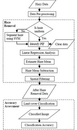
[image:3.612.370.494.510.718.2]Haze removal and performance assessment processes were then carried out. In dealing with non-uniform haze, there are additional steps need to be taken into account in implementing haze removal process, i.e. we need first to identify the haze uniformity. If haze is uniform, we can proceed carrying out the normal haze removal technique. If haze is not uniform, segmentation of haze need to be done accordingly so that every segment has almost homogenous haze and eventually haze removal can be applied to the individual segments.
121 Liang et al. [16] used unsupervised classification to separate haze by clustering the pixels to an optimum number of clusters based on haze severity and produced segments that consist of different haze levels. Nonetheless, there are drawbacks in unsupervised classification, such as it tends to produce classification with low accuracy and may cause over-clustering where pixels are clustered into inappropriate number of haze segments. In order to overcome this problem, we implement a different method that makes use of visual inspection and supervised classification to produce classification with higher accuracy.
In carrying out this procedure, bands 4, 3 and 2 were first displayed in red, green and blue channel since the haze effects is more apparent in these visible bands. The bands were analysed visually to identify different haze severity regions. Training pixels were selected from the different haze severity regions. Classification was performed using support vector machine (SVM), a supervised method, to classify the hazy data into two haze severity classes viz. severe and less severe. Masks were produced from the classified image and subsequently applied to the hazy data to produce severe and less severe segments of haze. Figure 3 shows the hazy data together with the masks. Eventually, each segment contains uniform haze where haze mean is subsequently to be calculated and subtracted from each segment before performing spatial filtering. PIF was used in order to determine haze mean for each segment.
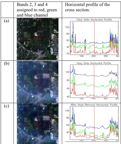
PIF were selected from both haze segments by selecting rooftops of residential and shop buildings. A linear regression relationship was then developed for the severe and less severe haze segments by making use of the PIFs from the hazy and clear data. The haze mean was subtracted from both haze segments for all bands. Subsequently, the severe and less severe haze from the hazy bands was combined where spatial filtering was next carried out. The hazy data dated from 19th September 2015 have moderate haze condition with 6 to 8km visibility. Higher classification accuracy was shown when implementing haze removal using spatial filter with kernel size 3x3 compared to 5x5. So, 3x3 kernel size was used for removing remaining noise due to haze variability. The accuracy differs mainly because the haze conditions in the simulated and real hazy data are different. In the simulated hazy data, the haze is homogenously distributed but in the real hazy data, the haze distribution is highly inhomogeneous. Figure 4 shows the true colour band combination of the clear and hazy data before and after haze removal side by side with the horizontal profile of the radiance value.
Visually, it can be seen that the data after haze removal shows less haze appearance compared to the data before haze removal. Besides that, the horizontal profile signifies that the radiance signatures for the data after haze removal were restored to almost similar to the radiance signatures of the clear data.
Masking band After mask data of
bands 2, 3 and 4 assigned to red, green and blue channel (a)
(b)
Figure 3: Masks (left) and The Corresponding Haze Segments (right) for (a) Severe Haze and (b) Less Severe Haze
Bands 2, 3 and 4 assigned to red, green and blue channel
Horizontal profile of the cross section.
(a)
(b)
(c)
[image:4.612.319.516.191.388.2] [image:4.612.312.522.432.682.2]122 4. ACCURACY ASSESSMENT
Haze removal has been carried out to remove the effects of haze from remote sensing data and consequently to improve the quality of the data. In order to evaluate the performance of the haze removal, accuracy assessment of the haze removal need to be carried out using suitable performance measures; here we make use visual analysis and classification accuracy.
4.1 Accuracy Assessment of Clear Data
Initially, land cover classification on clear data was carried out. There are three types of land cover identified, with oil palm as the major land cover followed by urban and forest. The oil palm plantation is located at nearly flat and hilly areas on the left and upper right part of the clear data respectively. The forest on the upper right of the clear data seems highly encroached for replacement with oil palm plantation. This produces an appearance of oil palm plantation on hilly area with mix cultivation area between forest and oil palm regions. On the other hand the forest on the lower right part of the clear image seems not being encroached for any agricultural activities.
The urban area is mainly part of Bandar Puncak Alam area which consists of residential areas, shop lots, universities, factories and warehouses. Two different sets of ROI were selected for training and reference purposes. Training pixels were selected from three land covers with 179 pixels for forest (red ROIs), 122 pixels for oil palm (green ROIs) and 116 for urban (blue ROIs). A different set of ROIs was then selected to be the reference pixels for each land cover. SVM was used to classify the land covers within the scene by making use of the training pixels. The pixels selection was done based on our experiences, and with the help Google Map [17]. Besides that we are used to Klang area and the type of plantation in the study area. In implementing this, we make use of skills in image interpretation to identify various features like tone, textures. Pattern, shape, size and analyse association of each
of the features [18]. The accuracy of the
classification was assessed via confusion matrix, by comparing the classification with the reference pixels. Figure 5 shows (a) clear data with band 4,3 and 2 assigned to red, green and blue channel and (b) classified image using training pixels. Visually, it can be seen that SVM successfully classify the pixels into the right classes with oil palm (51.1%) as the largest land cover, followed by urban (28.6%) and forest (20.3%). As stated before, there are mixed cultivation areas on the right part of the classified image consisting of patches of forest and oil palm. Confusion matrices were used to assess the accuracy of the classification with respect to the
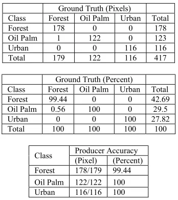
reference pixels. It can be seen that almost all pixels were rightly classified into the respective classes with only one pixel from forest is misclassified as oil palm. The overall accuracy of SVM classification for the clear data is 99.76% with kappa coefficient of 0.9963 (Table 2).
(a) (b)
Oil palm Urban Forest
[image:5.612.322.514.169.312.2]Figure 5: (a) Bands 4, 3 and 2 of The Clear Data Assigned to Red, Green and Blue Channel (b) The Classified Image of The Clear Data
Table 2. Confusion Matrix of The Clear Image in Terms of (a) Pixels, (b) Percent and (c) Producer Accuracy for
Each Class in Terms of Pixels and Percentages
Ground Truth (Pixels)
Class Forest Oil Palm Urban Total
Forest 178 0 0 178
Oil Palm 1 122 0 123
Urban 0 0 116 116
Total 179 122 116 417
Ground Truth (Percent)
Class Forest Oil Palm Urban Total
Forest 99.44 0 0 42.69
Oil Palm 0.56 100 0 29.5
Urban 0 0 100 27.82
Total 100 100 100 100
Class Producer Accuracy (Pixel) (Percent)
Forest 178/179 99.44
Oil Palm 122/122 100
Urban 116/116 100
Overall accuracy: 99.76% Kappa coefficient: 0.9963
(a) (b) (c)
[image:5.612.331.505.399.595.2] [image:5.612.318.531.618.700.2]123 4.2 Accuracy Assessment of Hazy Data
The same set of training pixels were used for the hazy data in order to carry out SVM classification. For the purpose of visual analysis, the classified images for the hazy data before and after haze removal are shown together side by side with the clear data in Figure 6. Obviously, it can be seen that there occur some pixels misclassification between oil palm and forest within the hazy data before undergoing haze removal. Some urban pixels are also misclassified as oil palm. The misclassifications tend to occur because the appearance of haze causes modification of the pixel radiance value recorded by the satellite due to haze scattering and absorption. The data after haze removal show visual quality improvement and higher classification accuracy.
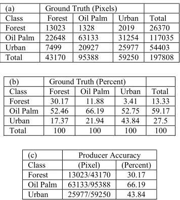
The misclassification between oil palm and forest seems have been reduced however not much improvement for the misclassification of urban area can be done by the haze removal. A clearer picture can be obtained by subsetting the classified image into a particular of interest in order to further analyse the hazy data after haze removal. The outcomes from subsetting the classified images to a smaller area of interest are shown in Figure 7. When making use the classification from the clear data as reference, the overall classification accuracy for the hazy data classification is 51.63% with kappa coefficient of 0.2 (Table 3). The producer accuracy for forest (30.17%), oil palm (66.19%), and urban (43.84%), is low, indicating that pixels misclassification is high for the hazy data. This is because haze layer has been affecting the radiance values (especially for bands 2, 3, and 4) and consequently causing a drop in the classification accuracy.
Table 4 displays the confusion matrix of the classified image for the data after haze removal. It shows that there is an increase of 31% in overall accuracy and an increase of 0.5 in Kappa coefficient. The overall accuracy and Kappa coefficient before after haze removal are 51.63% -82.62% and 0.2 - 0.7 respectively. This indicates that, the haze removal has successfully increased the classification accuracy of the hazy data. The producer accuracy for the classes is at acceptable and reliable level (i.e. 70% and above); for oil palm (87.18%) and urban (84.83%). Nonetheless, for forest (65.49%), the increase in producer accuracy is not up to the acceptable level since a large portion of the pixels were being misclassified as oil palm (33.56%) and urban (0.95%). In overall, the improvement of the classification is quite high and may be due to only three classes involved for this study area, resulting in a better restoration for the hazy data.
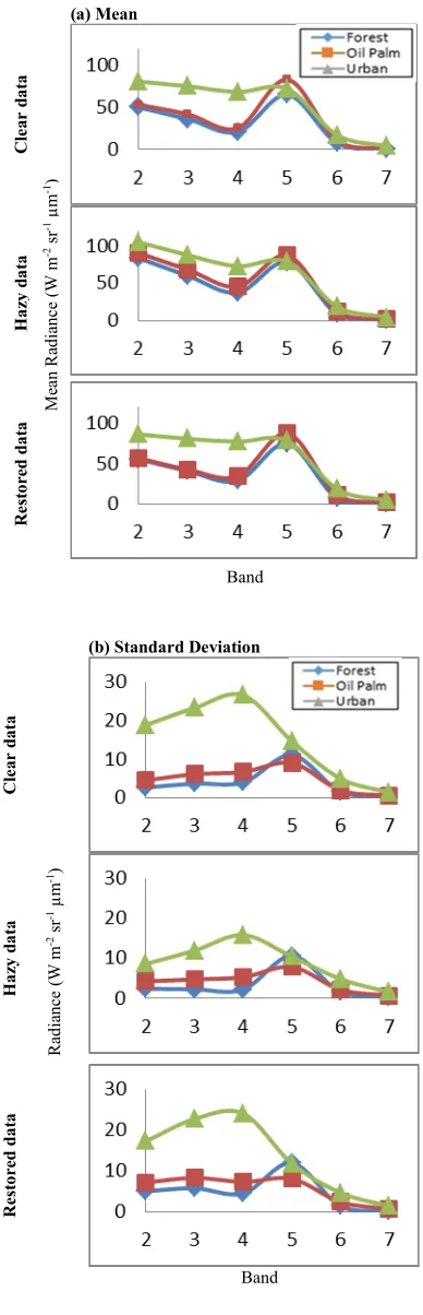
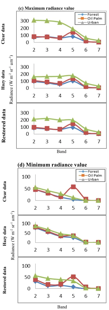
From the visual and classification accuracy analysis, the haze removal has successfully restored the spectral and statistical properties of the hazy data with respect to the clear data. Analysis on forest, oil palm and urban classes for clear, hazy and restored was done to examine the behaviour of their statistical and spectral properties. The statistical analysis covers the class mean, class standard deviation, class maximum and minimum value. All values are in radiance value
(W m-2 sr-1 µm-1) for each class and band. Figure 8
(a) shows mean radiance versus band for clear data, hazy data and hazy data after haze removal. By comparison there is a rise in class mean value for hazy data compared to class mean value for clear data. This is reasonable, because the effects of haze have modified the radiance values to new ones.
[image:6.612.314.527.288.431.2](a)
(b)
(c)
Figure 7: Subsetted Area of Classified Image of (a) Clear Data (b) Hazy Data (c )After Haze Removal Data
Table 3: Confusion Matrix of The Classified Image of Hazy Data with Respect to The Classified Image of The Clear Data In Terms of (a) Pixels, (b) Percent and (c) Producer Accuracy for
Each Class
(a) Ground Truth (Pixels)
Class Forest Oil Palm Urban Total
Forest 13023 1328 2019 26370
Oil Palm 22648 63133 31254 117035
Urban 7499 20927 25977 54403
Total 43170 95388 59250 197808
(b) Ground Truth (Percent)
Class Forest Oil Palm Urban Total
Forest 30.17 11.88 3.41 13.33
Oil Palm 52.46 66.19 52.75 59.17
Urban 17.37 21.94 43.84 27.5
Total 100 100 100 100
(c) Producer Accuracy
Class (Pixel) (Percent)
Forest 13023/43170 30.17
Oil Palm 63133/95388 66.19
Urban 25977/59250 43.84
[image:6.612.329.507.514.712.2]124
[image:7.612.319.513.125.727.2]Band
Table 4: Confusion Matrix of The Classification After Haze Removal With Respect to The Classification of The
Clear Data In Terms of (a) Pixels, (b) Percent and (c)
Producer Accuracy.
(a) Ground Truth (Pixel)
Class Forest Oil Palm Urban Total
Forest 29089 10709 177 39975
Oil Palm 14905 95879 9293 120077
Urban 422 3388 52966 56776
Total 44416 109976 62436 216828
(b) Ground Truth (Pixel)
Class Forest Oil Palm Urban Total
Forest 65.49 9.74 0.28 18.44
Oil Palm 33.56 87.18 14.88 55.38
Urban 0.95 3.08 84.83 26.18
Total 100 100 100 100
(c) Producer Accuracy
Class (Pixel) (Percent)
Forest 29089/44416 65.49
Oil Palm 95879/109976 87.18
Urban 52966/62436 84.83
Overall accuracy: 82.62%, Kappa coefficient: 0.70
Other than that, it can be seen that visible bands (2, 3 and 4) are more likely affected by haze than infrared bands (5, 6 and 7). This is because the visible bands record reflectance in shorter wavelengths and more likely to be affected by the suspended matter in the sky during hazy condition rather than the infrared bands that can partially penetrate certain concentrations of haze. If haze is too severe the infrared bands can also be affected. This is also due to the fact that at 6 to 8 km visibility the data is moderately affected by haze. Mean radiance for oil palm and forest are close to each other but still slightly different. This is because oil palm and forest possess vegetation features of green colour but still can be separate to different classes by SVM classifier. Since the mean values for infrared bands was not that affected by haze, only the mean values for visible bands will be further discussed. It can be seen that overall mean radiances for all classes after haze removal have approached the mean value of the clear data. This shows that the haze removal technique has preserved the radiance signature of the classes during clear condition.
Standard deviation is a measurement of variability of data with respect to the mean [19]. As illustrated in Figure 8 (b), it can be seen that standard deviation for urban area is high for visible bands (2, 3 and 4). This is because urban classes consist of mixed pixels of residential area, plants around the residential area, roads, pavements, industrial area and landscaping plants. Pixels with high and low radiances were classified together as
urban area resulting in higher standard deviation value.
(a) Mean
C
le
ar
d
at
a
M
ea
n
R
ad
ia
nc
e
(W
m
-2 s
r
-1 µ
m
-1)
H
az
y
da
ta
R
es
to
re
d
d
at
a
Band
(b) Standard Deviation
C
le
ar
d
at
a
R
ad
ia
nc
e
(W
m
-2 s
r
-1 µ
m
-1)
H
az
y
da
ta
R
es
to
re
d
d
at
a
125
Band
(c) Maximum radiance value
C
le
ar
d
at
a
R
ad
ia
nc
e
(W
m
-2 s
r
-1 µ
m
-1)
H
az
y
da
ta
R
es
to
re
d
d
at
a
Band
(d) Minimum radiance value
C
le
ar
d
at
a
R
ad
ia
nc
e
(W
m
-2 s
r
-1 µ
m
-1)
H
az
y
da
ta
R
es
to
re
d
d
at
a
Figure 8: (a) Mean, (b) Standard Deviation, (c) Maximum and (d) Minimum Radiance Value of Landsat Bands 2, 3, 4, 5, 6 and 7 For Forest, Oil Palm and Urban From Clear, Hazy and Restored
Data
On the other hand for oil palm and forest classes are mainly consist of pixels with low
radiances that lead to lower standard deviation for almost all bands except for band near infrared (band 5) since infrared bands are the best at detecting green vegetation pixels. Overall, it can be seen that the standard deviation for infrared bands are not that affected by haze than the visible bands [20]. The standard deviation for urban in visible bands drop drastically for hazy data as compared to clear data and is restored after haze removal.
Comparison for maximum and minimum value between clear, hazy and restored data is also important to monitor if there is overcorrection [21]. The plots for maximum and minimum value are shown in Figure 8 (c) and (d) respectively. Overall it can be seen that the maximum and minimum values also have the same behaviour as the mean and standard deviation since the data after haze removal have the properties close to the clear data.
4.3 Improvement of the haze removal compared to previous works
The haze removal proposed in this study made use the combination of absolute correction and image-based approach. Haze removal task can be carried out efficiently by making use minimum knowledge on haze condition. The accuracy of the developed haze removal has been tested via SVM classification accuracy.
5. CONCLUSION
We successfully a novel developed haze removal technique and applied it to real hazy data with inhomogeneous haze, located in Selangor, Malaysia. The performance evaluation shows that the technique is able to remove most haze within the scene although there is still observable haze appearance after the haze removal process. The reliability of the haze removal technique is supported by the spectral and statistical analyses carried out on the restored data.
[image:8.612.100.292.95.639.2]126 ACKNOWLEDGEMENT
We would like to thank Universiti Teknikal Malaysia Melaka (UTeM) for funding this study under the Malaysian Ministry of Higher Education Grant (FRGS/2/2014/ICT02/FTMK/02/F00245).
REFERENCES
[1] Hashim, M. and Kanniah, K. D. and Asmala,
A. and Rasib AW. Remote sensing of tropospheric pollutants originating from 1997 forest fire in Southeast Asia. Asian J Geoinformatics. 2004;4(4):57–67.
[2] Razali MF, Ahmad A, Mohd O, Bahari NIS, Sakidin H. Quantifying Haze from Satellite using Haze Optimized Transformation (HOT). Appl Math Sci 9(29):1407–16, 2015 [3] Morris W. The Heritage Illustrated Dictionary
of English Language of The English Language. New York : American Heritage Publishing Co. New York: American Heritage Publishing Co; 1975.
[4] Rahman HA, Effects AT, Haze O. Haze Phenomenon in Malaysia : Domestic or Transboudry Factor ?;597–9, 2013
[5] Ahmad A, Quegan S. The effects of haze on the spectral and statistical properties of land cover classification. Appl Math Sci. 8(180):9001–13, 2014
[6] Ahmad A, Quegan S. The Effects of Haze on the Accuracy of Satellite Land Cover
Classification. Appl Math Sci.
2015;9(49):2433–43.
[7] Morisette JT, Shuey CJ, Walthall CL, Daughtry CST. Atmospheric correction of Landsat ETM+ land surface imagery. II. Validation and applications. IEEE Trans Geosci Remote Sens. Dec;40(12):2736–46, 2002
[8] Zhang Y, Guindon B. Quantitative
Assessment of a Haze Suppression
Methodology for Satellite Imagery : Effect on Land Cover Classification Performance. IEEE Trans Geosci Remote Sens. 41(5):1082–9, 2003
[9] Chavez PS. An improved dark-object
subtraction technique for atmospheric
scattering correction of multispectral data. Remote Sens Environ. 24(3):459–79, 1988 [10] Moro GD, Halounova L. Haze removal for
high‐resolution satellite data: a case study. Int
J Remote Sens. 28(10):2187–205, 2007 [11] Hu J, Chen W, Li X, He X. A haze removal
module for mutlispectral satellite imagery. 2009
[12] Hu C, Tang P. Converting DN value to reflectance directly by relative radiometric normalization. Proc - 4th Int Congr Image Signal Process CISP 2011. 3:1614–8, 2011 [13] Alberts K. Landsat 8 (L8) Level 1 (L1) Data
Format Control Book (DFCB). 2015.
[14] Roy DP, Wulder M a., Loveland TR, C.E. W, Allen RG, Anderson MC, et al. Landsat-8: Science and product vision for terrestrial global change research. Remote Sens Environ.;145:154–72, 2014
[15] USGS. USGS [Internet]. 2015 [cited 2015
Apr 22]. Available from:
http://glovis.usgs.gov/
16. Liang S, Member S, Fang H, Chen M. Atmospheric Correction of Landsat ETM + Land Surface Imagery — Part I : Methods.
IEEE Trans Geosci Remote Sens.
39(11):2490–8, 2001
[17] GoogleMaps. Google Maps [Internet]. 2015. Available from:
https://www.google.com.my/maps
[18] N. McWilliam, R. Teeuw MW and PZ. Field Techniques Manual: GIS, GPS and Remote Sensing. F Tech Man GIS, GPS Remote Sens. 68–76, 2005
[19] Bluman AG. Elementary Statistics: A Step By Step Approach. 7th ed. New York:
McGraw-Hill; 604 p, 2007
[20] Ahmad and S. Quegan. Haze modelling and
simulation in remote sensing satellite data,
Applied Mathematical Sciences,
8(159):7909–7921, 2014
[21] A. Ahmad, Mohd Khanapi Abdul Ghani,