Genotype free demultiplexing of pooled single cell RNA seq

M E T H O D

Open Access

Genotype-free demultiplexing of

pooled single-cell RNA-seq

Jun Xu

, Caitlin Falconer

, Quan Nguyen

, Joanna Crawford

, Brett D. McKinnon

, Sally Mortlock

,

Anne Senabouth

, Stacey Andersen

, Han Sheng Chiu

, Longda Jiang

, Nathan J. Palpant

,

Jian Yang

, Michael D. Mueller

, Alex W. Hewitt

, Alice Pébay

, Grant W. Montgomery

,

Joseph E. Powell

and Lachlan J.M Coin

Abstract

A variety of methods have been developed to demultiplex pooled samples in a single cell RNA sequencing

(scRNA-seq) experiment which either require hashtag barcodes or sample genotypes prior to pooling. We introduce scSplit which utilizes genetic differences inferred from scRNA-seq data alone to demultiplex pooled samples. scSplit also enables mapping clusters to original samples. Using simulated, merged, and pooled multi-individual datasets, we show that scSplit prediction is highly concordant with demuxlet predictions and is highly consistent with the known truth in cell-hashing dataset. scSplit is ideally suited to samples without external genotype information and is available at:https://github.com/jon-xu/scSplit

Keywords: scSplit, scRNA-seq, Demultiplexing, Machine learning, Unsupervised, Hidden Markov Model, Expectation-maximization, Genotype-free, Allele fraction, Doublets

Background

Using single-cell RNA sequencing (scRNA-seq) to cell biology at cellular level provides greater resolution than “bulk” level analyses, thus allowing more refined under-standing of cellular heterogeneity. For example, it can be used to cluster cells into sub-populations based on their differential gene expression, so that different fates of cells during development can be discovered. Droplet-based scRNA-seq (for example Drop-Seq [1] or 10X Genomics Systems [2]) allows profiling large numbers of cells for sequencing by dispersing liquid droplets in a continuous oil phase [3]s in an automated microfluidics system, and as a result is currently the most popular approach to scRNA-seq despite a high cost per run. Methods that lower the per sample cost of running scRNA-seq are required in order to scale this approach up to a population scale. An effective method for lowering scRNA-seq cost is to pool

*Correspondence:lachlan.coin@unimelb.edu.au

1_{Genome Innovation Hub, The University of Queensland, 306 Carmody Road,} St Lucia, QLD 4072 Brisbane, Australia

2_{Institute for Molecular Bioscience, The University of Queensland, 306} Carmody Road, St Lucia, QLD 4072 Brisbane, Australia

Full list of author information is available at the end of the article

samples prior to droplet-based barcoding with subsequent demultiplexing of sequence reads.

Cell hashing [4] based on Cite-seq [5] is one such exper-imental approach to demultiplex pooled samples. This approach uses oligo-tagged antibodies to label cells prior to mixing, but use of these antibodies increases both the cost and sample preparation time per run. More-over, it requires access to universal antibodies for organ-ism of interest, thus limiting applicability at this stage to human and mouse. Alternatively, computational tools like demuxlet [6] have been developed to demultiplex cells from multiple individuals, although this requires addi-tional genotyping information to assign individual cells back to their samples of origin. This limits the utility of demuxlet, as genotype data might not be available for dif-ferent species; biological material may not be available to extract DNA; or the genetic differences between samples might be somatic in origin.

Another issue for droplet-based scRNA-seq protocols is the presence of doublets, which occurs when two cells are encapsulated in same droplet and acquire the same bar-code. The proportion of doublets increases with increas-ing number of cells barcoded in a run. It is imperative that

Xuet al. Genome Biology (2019) 20:290 Page 2 of 12

these are flagged and removed prior to downstream anal-ysis. Demuxlet [6] uses external genotype information to address this issue, and other tools have been developed to solve this issue based on expression data alone, including Scrublet [7] and Doubletfinder [8].

Here we introduce a simple, accurate, and effi-cient tool, mainly for droplet-based scRNA-seq, called "scSplit", which uses a hidden state model approach to demultiplex individual samples from mixed scRNA-seq data with high accuracy. Our approach does not require genotype information from the individual sam-ples to demultiplex them, which also makes it suit-able for applications where genotypes are unavailsuit-able or difficult to obtain. scSplit uses existing bioinfor-matics tools to identify putative variant sites from scRNA-seq data, then models the allelic counts to assign cells to clusters using an expectation-maximisation framework.

Results

Our new tool, scSplit for demultiplexing pooled sam-ples from scRNA-seq data, only requires the FASTQ files obtained from single cell sequencing, together with a white-list of barcodes, while it does not require genotype data, nor a list of common variants if not available. Result data are available in https://github.com/jon-xu/scSplit_ paper_data.

Simulation run showed high accuracy and efficiency of scSplit

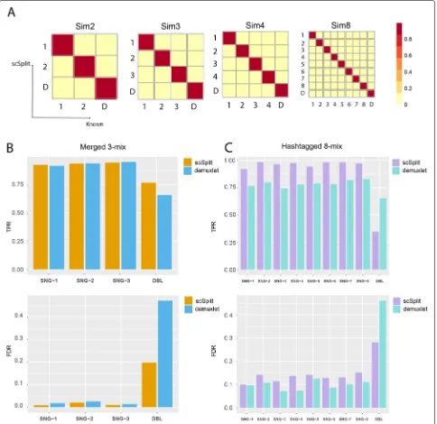
We used a single scRNA-seq BAM file from Zheng et al. [2] as a template for simulation. Additionally, we took 32 samples from genoptype information used in figure 2 supplementary data of Kang et al. [6], as the source of multi-sample genotype likelihoods for simulation (see “Data simulation” inMethods). We ran simulation tests using our scSplit tool and used the distinguishing vari-ants to identify the individual donor for each cluster. In order to assess the accuracy of the method, we cal-culated both the proportion of cells from each cluster which were correctly assigned to it among the true cor-rect number of cells in each cluster (True Positive Rate or TPR), as well as the proportion of cells assigned to a cluster which were incorrect against the total assigned cells (false discovery rate or FDR). We also report the average TPR and average FDR. We obtained very high overall TPR (0.97) and low FDR (less than 1e−4) for from 2- to 32-mixed samples, with very accurate dou-blet predictions (Table 1, Fig. 1a). To test the limit of our tool on genotype difference, we downloaded three pairs of full sibling genotypes from the UK Biobank and simulated pooled samples by mixing one pair at a time, the average singlet TPR was beyond 0.87 (Table S2 in Additional file2).

scSplit performed similarly well to demuxlet in demultiplexing merged individually sequenced three stromal samples

We then tried running scSplit on a manual merging of three individually sequenced samples. We merged the BAM files from three individual samples (Methods). In order to create synthetic doublets, we randomly chose 500 barcodes whose reads were merged with another 500 barcodes. We ended up with 9067 singlets and 500 doublets, knowing their sample origins prior to merging. Both scSplit and demuxlet [6] pipelines were run on the merged samples, and the results were compared with the known individual sample data. We observed high concor-dance of singlet prediction between both tools (TPR/FDR: 0.94/0.02 vs 0.93/0.02), and a better doublet prediction from scSplit compared to demuxlet (TPR/FDR: 0.65/0.04 vs 0.66/0.47) (Fig.1b and Table2). We then downsampled the mixed sample to 2800 reads per cell in order to test the performance under low sequencing depth and the over-all result was still good (TPR = 0.91, FDR = 0.03), which indicated that scSplit can work under shallow read depth.

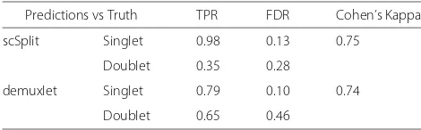
scSplit predictions highly consistent with known source of hashtagged and pooled eight PBMC samples

Next, we tested scSplit on a published scRNA-seq dataset (GSE108313) which used cell-hashing technology to mark samples of the cells before multiplexing [4]. We ran through the scSplit pipeline with the SNVs filtered by common SNVs provided on The International Genome Sample Resource (IGSR) [9].

According to the scSplit pipeline, distinguishing vari-ants were identified, and the P/A matrix was generated to assign the cells to clusters (Methods). We then extracted the reference and alternative allele absence information at these distinguishing variants from the sample genotypes and generated a similar P/A matrix. Both matrices were compared so that clusters were mapped to samples (Figure S1 in Additional file1).

Our results were highly consistent with the known cell hashing tags (Table 3). We saw higher TPR for singlets in scSplit (0.98) than demuxlet (0.79) and similar singlet FDRs (0.10 vs 0.13). Although the doublet TPR of scSplit (0.35) was lower than for demuxlet (0.65), the doublet FDR (0.28) was better than demuxlet (0.46). If the expected number of doublets was selected higher, cells with largest read depth could be moved from singlet clusters to the doublet cluster to increase the TPR for doublets with a decrease of TPR for singlets.

Table 1Overview of accuracy and performance of scSplit on simulated mixed samples, with one CPU and 30GB RAM

Simulation sim2 sim3 sim4 sim8 sim12 sim16 sim24 sim32

Mixed samples 2 3 4 8 12 16 24 32

Number of cells 12 383 12 383 12 383 12 383 12 383 12 383 12 383 12 383

Reads per cell 4 973 4 973 4 973 4 973 4 973 4 973 4 973 4 973

Informative SNVs 34 116 34 116 34 116 34 116 34 116 34 116 34 116 34 116

Assigning cells 41 min 41 min 46 min 47 min 1h54m 2h11 2h33 2h55

Singlet TPR 0.97 0.97 0.97 0.97 0.97 0.97 0.96 0.96

Singlet FDR 0 9E−5 9E−5 9E−5 0 0 5E−3 8E−3

Doublet TPR 0.997 0.997 0.997 0.997 0.997 0.997 0.995 0.997

Doublet FDR 0 0 0 0 0 0 0 0

Cohen’s Kappa 1.0 1.0 1.0 1.0 1.0 1.0 0.97 0.98

We used PBMC donor B [2] and genotype data from demuxlet [6] as simulation templates

have good concordance with sample genotypes (Table S1 in Additional file2).

Comparing scSplit with demuxlet on more pooled scRNA-seq samples

We ran scSplit with common SNV filtering on published data from the demuxlet paper [6]. By taking demuxlet pre-dictions as ground truth, we achieved high singlet TPR (0.80), although the doublet prediction of the two tools were quite distinct to each other (Fig.2a and Table4).

We also ran our tool on a set of genotyped and then pooled fibroblast scRNA-seq datasets. Predictions from scSplit and demuxlet showed high concordance in singlet prediction (TPR: 0.93–0.94, FDR: 0.06–0.07), although not on doublets (TPR: 0.08–0.52, FDR: 0.45–0.92) when demuxlet was treated as gold standard (Fig. 2b and Table 5). Mapping between clusters and samples were recorded (Figure S2 in Additional file1).

Pooling samples together showed similar effects as normalizing individually sequenced samples

We further checked the gene expression profiles of the previously illustrated three individual stromal samples (Fig. 1b and Table 2). We plotted Uniform Manifold Approximation and Projection for Dimension Reduction (UMAP) [10] for non-pooled and pooled scenarios with and without normalization. The samples were more sepa-rated from each other in non-pooled and non-normalized scenario (Fig.3a), and got less distant for other scenar-ios including non-pooled but normalized (Fig.3b), pooled and non-normalized (Fig.3c), and pooled and normalized (Fig.3d). We calculated Silhouette values for each of the UMAPs and got 0.28 for Fig.3a, 0.12 for Fig.3b, 0.14 for Fig.3c, and 0.19 for Fig. 3d. As bigger Silhouette values indicate larger difference between samples, we could say both normalization and pooling could reduce the batch effects between individually sequenced samples. However,

by pooling samples together for sequencing could mini-mize the potential information loss during normalization.

Discussion

We developed the scSplit toolset to facilitate accurate, cheap, and fast demultiplexing of mixed scRNA samples, without needing sample genotypes prior to mixing. scSplit also generates a minimum set of alleles (as few as the sample numbers), enabling researchers to link the result-ing clusters with the actual samples by comparresult-ing the allele presence at these distinguishing loci. When prede-fined individual genotypes are not available as a reference, this can be achieved by designing a simple assay focused on these distinguishing variants (such as a Massarray or multiplexed PCR assay). Although the tool was mainly designed for droplet-based scRNA-seq, it can also be used for scRNA-seq data generated from other types of scRNA-seq protocols.

We filtered out indels, MNPs, and complex rearrange-ments when building the model and were able to show that SNVs alone provide adequate information to delineate the differences between multiple samples. As an alterna-tive to using allele fractions to model multiple samples, genotype likelihoods could also be used for the same pur-pose; however, more memory and running time would likely be needed, especially when barcode numbers in mixed sample experiments increase. Our tests showed no discernable difference in accuracy between these two methods.

Xuet al. Genome Biology (2019) 20:290 Page 4 of 12

Fig. 1Results on simulated, merged hash-tagged scRNA-seq datasets confirmed scSplit a useful tool to demultiplex pooled single cells.aConfusion matrix showing scSplit demultiplexing results on simulated 2-, 3-, 4- and 8-mix;bTPR and FDR of for singlets and doublets predicted by scSplit and demuxlet compared to known truth before merging;cTPR and FDR of for singlets and doublets predicted by scSplit and demuxlet compared to cell hashing tags

sample number. Further optimization of the tool would be needed to effectively implement these options.

Although scSplit was mainly tested on human samples, it can also be applied to other organisms and is espe-cially useful for those species without dense genotyping chips available. We also expect the application of scSplit in cancer -related studies, to distinguish tumor cells from healthy cells, as well as to distinguish tumor sub-clones.

Conclusions

Table 2Comparison of scSplit and demuxlet performance in demultiplexing merged three individually genotyped stromal samples (TPRtrue positive rate,FDRfalse discovery rate); Total cell numbers: 9567; Reads per cell: 14,495; Informative SNVs: 63,129; Runtime for matrices building: 67 min, Runtime for cell assignment: 55 min

Predictions vs Truth TPR FDR Cohen’s Kappa

scSplit Singlet 0.94 0.02 0.95

Doublet 0.65 0.04

demuxlet Singlet 0.93 0.02 0.77

Doublet 0.66 0.47

infections, delineating tumor sub-clones and sequence analysis in non-model organisms.

Methods

All relevant source code is available athttps://github.com/ jon-xu/scSplit/.

Overview

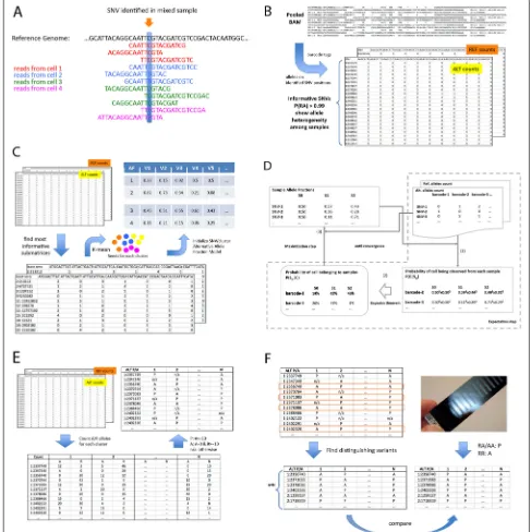
The overall pipeline for the scSplit tool includes seven major steps (Fig.4):

1 Data quality control and filtering: The mixed sample BAM file is first filtered to keep only the reads with a list of valid barcodes to reduce technical noise. Additional filtering is then performed to remove reads that meet any of the following: mapping quality score less than 10, unmapped, failing quality checks, secondary or supplementary alignment, or PCR or optical duplicate. The BAM file is then marked for duplication, sorted and indexed.

2 SNV calling (Fig.4a): Freebayes v1.2 [11] is used to call SNVs on the filtered BAM file, set to ignore insertions and deletions (indels), multi-nucleotide polymorphisms (MNPs), and complex events. A minimum base quality score of one and minimum allele count of two is required to call a variant. The output VCF file is further filtered to keep only SNVs with quality scores greater than 30.

Table 3Comparison of scSplit and demuxlet performance in demultiplexing hashtagged and multiplexed eight individually genotyped PBMC samples (TPRtrue positive rate,FDRfalse discovery rate); total cell numbers: 7932; reads per cell: 5835; informative SNVs: 16,058; runtime for matrices building: 35 min, runtime for cell assignment: 20 min

Predictions vs Truth TPR FDR Cohen’s Kappa

scSplit Singlet 0.98 0.13 0.75

Doublet 0.35 0.28

demuxlet Singlet 0.79 0.10 0.74

Doublet 0.65 0.46

3 Building allele count matrices (Fig.4b): The “matrices.py” script is run which produces two .csv files, one for each of reference and alternate allele counts as output.

4 Model initialization (Fig.4c): find the distinct groups of cells in the scRNA-seq and use them to initialize the Allele Fraction Model (SNVs by samples). 5 E-M iterations till convergence (Fig.4d): Initialized

allele fraction model and the two allele count

matrices are used together to calculate the probability of each cell belonging to the clusters. After each round, allele fraction model is updated based on the probability of cell assignment and this is iterated until overall likelihood of the model reaches convergence. 6 Alternative presence/absence genotypes (Fig.4e):

matrix indicating cluster genotypes at each SNV is built in this step.

7 Find distinguishing variants for clusters and use to assign samples to clusters (Fig.4f): In order to assign each model cluster back to the specific sample, distinguishing variants are identified so that genotyping of the least number of loci using the a suitable platform may be performed. Gram-Schmidt orthogonalization [12] is used to get the minimum set of informative P/A genotypes.

Data quality control

Samtools was used to filter the reads with verified bar-codes for mapping and alignment status, mapping quality, and duplication (samtools view -S -bh -q 10 -F 3844 [input] >[output]). Duplicates were removed (samtools rmdup [input] [output]) followed by sorting and indexing.

SNV calling on scRNA-seq dataset

SNVs were called on the scRNA-seq mixed sample BAM file with freebayes [11], a widely used variant calling tool. The freebayes arguments “-iXu -q 1” were set to ignore indels and MNPs and exclude alleles with support-ing base quality scores of less than one. This generated a VCF file containing all SNVs from the mixed sample BAM file. Common SNPs of a population (for example results from The international Genome Sample Resource [9]) were recommended be used to filter out noisy SNVs.

Building allele count matrices

Xuet al. Genome Biology (2019) 20:290 Page 6 of 12

Fig. 2Results of scSplit on pooled PBMC scRNA-seq and that on a set of pooled fibroblast samples.aSinglet TPR and FDR compared to demuxlet predictions on pooled PBMC scRNA-seq.bViolin plot of singlet TPR and FDR for five 7- or 8-mixed samples based on scSplit vs demuxlet

position. This provided a full map of the distribution of reference and alternate alleles across all barcodes at each SNV.

The allele count matrices captured information from all reads overlapping SNVs to reflect the different allele fraction patterns from different barcodes or samples. To build the allele count matrices, pysam fetch [13] was used to extract reads from the BAM file. The reads overlap-ping each SNV position were fetched and counted for the presence of the reference or alternate allele. In order to increase overall accuracy and efficiency, SNVs whose GL(RA) (likelihood of heterozygous genotypes) was lower

Table 4Comparison of scSplit and demuxlet performance in demultiplexing multiplexed eight individually genotyped PBMC samples (TPRtrue positive rate,FDRfalse discovery rate); total cell numbers: 6145; reads per cell: 33,119; informative SNVs: 22,757; runtime for matrices building: 45 min; runtime for cell assignment: 35 min

scSplit vs demuxlet TPR FDR Cohen’s Kappa

Singlets 0.80 0.18 0.63

Doublets 0.12 0.92

than log₁₀(1 − error) where error = 0.01 were filtered out. These were more homozygous and thus less infor-mative for detecting the differences between the multiple samples. The generated matrices were exported

Table 5Overview of accuracy and performance running scSplit on five multiplexed scRNA-seq datasets, with one CPU and 30 GB RAM

scSplit vs demuxlet Mix 1 Mix 2 Mix 3 Mix 4 Mix 5

Mixed samples 7 8 8 8 7

Number of cells 914 8 137 5 165 6 977 7 428

Reads per cell 86 148 16 386 21 265 18 572 19 657

informative SNVs 15 848 26 830 26 162 23 224 41 993

Build matrices 10 min 23 min 18 min 21 min 35 min

Assign cells 4 min 47 min 23 min 45 min 50 min

Singlet TPR 0.94 0.93 0.94 0.93 0.93

Singlet FDR 0.06 0.07 0.06 0.07 0.07

Doublet TPR 0.52 0.17 0.15 0.17 0.08

Doublet FDR 0.48 0.83 0.85 0.83 0.92

Cohen’s Kappa 0.86 0.78 0.68 0.77 0.76

Fig. 3Batch effect during sequencing runs found in comparison of individual runs was obvious compared to that in pooled scRNA-seq data.a UMAP for three individually sequenced samples.bUMAP for three individually sequenced and normalized samples.cUMAP for pooled sequencing of same three individual samples, samples marked based on demultiplexing results using scSplit.dUMAP for pooled sequencing of same three individual samples, normalized by total sample reads

Model initialization by using maximally informative cluster representatives

To initialize the model, initial probabilities of observing an alternative allele on each SNV position in each clus-ter were calculated. The overall matrix was sparse and a dense sub-matrix with a small number of zero count cells was generated. To do that, cells were first sorted accord-ing to their number of zero allele counts (sum of reference and alternative alleles) at all SNVs and SNVs were simi-larly sorted according to their number of zero allele counts (sum of reference and alternative alleles) across all cells. Next, we selected and filtered out 10% of the cells among those with the most number of zero expressed SNVs and 10% of the SNVs among those where the most number cells had zero counts. This was repeated until all remain-ing cells had more than 90% of their SNVs with non-zero allele counts and all SNVs had non-zero counts in more than 90% of cells. This subset of matrices was the basis for the seed barcodes to initialize the whole model. The

sub-matrix was transformed using PCA with reduced dimensions and then K-means clustering was performed to split the cell subset into expected number of clusters. By using the allele fractions on the subset of SNVs in these initially assigned cells, each cluster of the model could be initialized. LetN(Ac,v)andN(Rc,v)be the Alternative

and Reference allele counts on SNVvand cellc accord-ingly, and let pseudoAR be the pseudo allele count for

both Alternative and Reference alleles, and pseudoAbe the

pseudo allele count for Alternative alleles, we calculated

P(Av|Sn), the probability of observing Alternative allele on

SNVvin Samplen, according to below equation:

P(Av|Sn)=

c

N(Ac,v)+pseudoA)

c

N(Ac,v)+ c

N(Rc,v)+pseudoAR

Xuet al. Genome Biology (2019) 20:290 Page 8 of 12

Fig. 4The overall pipeline of scSplit tool.aSNV identified based on reads from all cells which have similar or different genotypes.bAlternative and reference allele count matrices built from each read in the pooled-sequenced BAM at the identified informative SNVs.cInitial allele fraction model constructed from the initial cell seeds and their allele counts.dExpectation-maximization process to find the most optimized allele fraction model, based on which the cells are assigned to clusters.ePresence/Absence matrix of alternative alleles generated from the cell assignments.fMinimum set of distinguishing variants found to be used to map clusters with samples

We also initiated the probability of seeing thenth sam-ple as evenly distributed across all samsam-ples. LetP(Sn)be

the probability of seeing then-th sample, andN(S)be the number of samples to be demultiplexed:

P(Sn)=

1

N(S) (2)

Expectation–maximization approach

the allele fraction model. EM iterations stopped when convergence was reached, so that the overall probability of observing the cells, or the reference/alternative alleles count matrices, was maximized.

During the E-step, the tool first calculated P(Ci|Sn),

the likelihood of observing a cellCi in sampleSn, which

was equal to the product of the probability of observing the allele fraction pattern over each SNV, which in turn equaled to the product of probability of having observed the count of alternative alleles and probability of having observed the count of reference alleles. Letcibe the i-th

cell,Snbe the n-th sample,Avbe the Alternative allele on

SNV v, and N(A), N(R) be the quantity of Alternative and Reference alleles:

P(Ci|Sn)=P(Aci,Rci|Sn)

=

v

P(Av|Sn)N(Aci,v)[ 1−P(Av|Sn)]N(Rci,v)

(3)

And then P(Ci|Sn) was transformed to P(Sn|Ci), the

cell-sample probability, i.e. the probability of a cell Ci

belonging to sampleSn, using Bayes’ theorem, assuming

equal sample prior probabilities (P(S1) = P(S2) = ... =

P(Sn)):

P(Sn|Ci)=

P(Ci|Sn) N

x=1

P(Ci|Sx)

(4)

Next, weighted allele counts were distributed to the dif-ferent cluster models according to the cell-sample prob-ability, followed by the M-step, where the allele fraction model represented by the alternative allele fractions was updated using the newly distributed allele counts, so that allele fractions at all SNV positions in each sample model were recalculated:

P(Av|Sn)=

i

N(Ac,v)P(Sn|Ci)+pseudoA

i

N(Tc,v)P(Sn|Ci)+pseudoAR

(5)

And the sample probabilityP(Sn) was also updated by

the newly calculated cell likelihoods:

P(Sn)=

i

P(Sn|Ci)

n

i

P(Sn|Ci)

(6)

The overall log-likelihood of the whole model [15] was calculated as:

Lmodel=

i

log

n

P(Ci|Sn)

= i log n v

P(Ci,v|Sn,v)P(Sn)

(7)

Multiple runs to avoid local maximum likelihood

The entire process was repeated for 30 rounds with the addition of randomness during model initialization and the round with the largest sum of log likelihood was taken as the final result. Randomness was introduced by ran-domly selecting the 10% of cells and SNVs to be removed from the matrices during initialization from a range of the lowest ranked cells and SNVs as detailed previously.

Cell cluster assignment

Next, probability of a cell belonging to a clusterP(Sn|Ci)

was calculated. Cells were assigned to a cluster based on a minimum threshold of P > 0.99. Those cells with no P(Sn|Ci) larger than the threshold were regarded as

unassigned.

Handling of doublets

During scRNA-seq experiments, a small proportion of droplets can contain cells from more than one sample. These so called doublets, contain cells from same or dif-ferent samples sharing the same barcode, which if not addressed would cause bias. Our model took these dou-blets into consideration. During our hidden state based demultiplexing approach, we included an additional clus-ter so that doublets could be captured. To identify which cluster in the model was the doublet cluster in each round, the sum of log-likelihood of cross assignments was checked:

P(c isdoublet)=

i∈/c

v

P(Ci,v|Sc,v)P(Sc) (8)

The sum log-likelihood of cells from all other clusters being assigned to a specific cluster was calculated for each cluster in turn and compared. The cluster with the largest sum log-likelihood of cross assignment was designated as the doublet cluster. We allow user input on the expected proportion of doublets. If the expected number of dou-blets was larger than those detected in the doublet cluster, cells with largest read depth were moved from singlet clus-ters to doublet cluster, so that the total number of doublets meet expectation as input.

Alternative allele presence/absence genotyping for clusters

Xuet al. Genome Biology (2019) 20:290 Page 10 of 12

Mapping clusters back to individual samples using minimal set of P/A genotypes

Based on the P/A matrix, we started from informative SNVs which had variations of “P” or “A” across clusters and avoid picking those with “NAs”. Then, unique patterns involved in those SNVs were derived and for each unique P/A pattern, one allele was selected to subset the whole matrix. Next, Gram-Schmidt orthogonalization [12] was applied on the subset of P/A matrix, in order to find the variants which can be basis vectors to effectively distin-guish the clusters. If not enough SNVs were found to distinguish all the clusters, the clusters were split into smaller groups so that for each group there was enough variants to distinguish the clusters within that group. And to distinguish clusters from different smaller groups, if the selected variants could not be used to distinguish any pair of clusters, additional variants were selected from the whole list of variants where no NAs were involved and P/A was different between the pair of clusters. Ideal situation was N variants for N clusters, but it was possible that>N variants were needed to distinguish N clusters.

As such, the P/A genotyping of each cluster, on the minimum set of distinguishing variants, could be used as a reference to map samples to clusters. After run-ning genotyping on this minimum set of loci for each of the individual samples, a similar matrix based on sample genotypes could be generated, by setting the alternative presence flag when genotype probability (GP) was larger than 0.9 for RA or AA, or absence flag when GP was larger than 0.9 for RR. By comparing both P/A matrices, we could link the identified clusters in scSplit results to the actual individual samples.

In practice, samples can be genotyped only on the few distinguishing variants, so that scSplit-predicted clusters can be mapped with individual samples, while the whole genotyping is not needed. When the whole genotyping is available, we also provide an option for users to gen-erate distinguishing variants only from variants with R2

>0.9, so that they can compare the distinguishing matrix from scSplit with that from known genotypes on more confident variants.

Data simulation

To test the consistency of the model, and the perfor-mance of our demultiplexing tool, reference/alternative count matrices were simulated from a randomly selected scRNA-seq BAM file from Zheng et al. [2] and a 32-sample VCF file used in Fig. 2 supplementary data of Kang et al. [6]. We assume the randomly selected BAM file had a representative gene expression profile.

First, data quality was checked and the BAM and VCF files were filtered. Second, barcodes contained in the BAM file were randomly assigned to samples in the VCF file, which gave us the gold-standard of cell-sample

assignments to check against after demultiplexing. Then, all the reads in the BAM file were processed, that if a read overlapped with any SNV position contained in the merged VCF file, its barcode was checked to get its assigned sample and the probabilityP(Ac,v)of having the

alternative allele for that sample was calculated using the logarithm-transformed genotype likelihood (GL) or geno-type probability (GP) contained in the VCF file. The prob-ability of an allele being present at that position could then be derived so that the ALT/REF count at the SNV/barcode in the matrices could be simulated based on the alternative allele probability. LetL(AA)andL(RA)be the likelihood of seeing AA and RA of a certain cell c on a certain SNV v:

P(Ac,v)=

1 210

[log₁₀L(RA)]₊₁₀[log₁₀L(AA)] ₍₉₎

Finally, doublets were simulated by merging randomly chosen 3% barcodes with another 3% without overlap-ping in the matrix. This was repeated for every single read in the BAM file. This simulation modeled the number of reads mapped to the reference and alternative alleles directly. In our simulations, there were 61 576 853 reads in the template BAM file for 12 383 cells, which was equivalent to 4973 rpc.

With the simulated allele fraction matrices, the bar-codes were demultiplexed using scSplit and the results were compared with the original random barcode sample assignments to validate.

Result evaluation

We used both TPR/FDR and Cohen’s Kappa [16] to eval-uate the demultiplexing results against ground truth. R package “cluster” [17] was used in evaluating the clusters on UMAPs in Fig.3.

Single cell RNA-seq data used in testing scSplit

In Tables3and4, we used published hashtagged data from GSE108313 and PBMC data from GSE96583. For Tables2

and5, endometrial stromal cells cultured from 3 women and fibroblast cells cultured from 38 healthy donors over the age of 18 years respectively were run through the 10x Genomics Chromium 3’ scRNA-seq protocol. The libraries were sequenced on the Illumina Nextseq 500. FASTQ files were generated and aligned to Homo sapiens GRCh38p10 using Cell Ranger. Individuals were geno-typed prior to pooling using the Infinium PsychArray.

Full sibling data from UK biobank used in simulation

Supplementary information

Supplementary informationaccompanies this paper at https://doi.org/10.1186/s13059-019-1852-7.

Additional file 1:Figure S1. Illustration of presence absence matrices calculated on pooled and hashtagged scRNA-seq datasets.Figure S2. Illustration of presence absence matrices calculated on pooled fibroblast scRNA-seq datasets.

Additional file 2:Table S1. Accuracy of alternative allele Presence/Absence genotypes built from scSplit/demuxlet clusters compared with that from sample genotyping, based on Hashtag scRNA-seq dataset.Table S2. Simulation using full sibling genotypes from UK Biobank shows scSplit can work for very closely related pooled samples. Additional file 3:Review history.

Additional information

Peer review information: Barbara Cheifet was the primary editor on this article and managed its editorial process and peer review in collaboration with the rest of the editorial team.

Acknowledgements

We thank Rahul Satija and Shiwei Zheng for providing helpful data from CITE-Seq based hashtagged scRNA-seq study [4]. And we appreciate Yang Ou’s support on scRNA-seq normalization. This research has been conducted using the UK Biobank Resource under Application Number ’12514’.

Review history

The review history is available as Additional file3.

Authors’ contributions

LC and CF initiated the project. LC and JX designed the algorithms. JX implemented the tools in Python and tested it on multiple datasets. MDM generated the endometrial stromal samples. AP and AH generated the fibroblast samples. QN, SM and AS preprocessed the sample datasets. JY and LJ provided the sibling data for simulation and helped in analysis. JP, QN, GWM, BM, SM, JC, and SA participated in important discussions and provided useful suggestions on multiple issues. JX drafted the manuscript, LC, JP, GWM, JY, QN, and JC reviewed and revised the manuscript. All authors read and approved the final manuscript.

Authors’ information

Jun Xu: Twitter(@xujun_jon) Lachlan J.M Coin: Twitter(@lachlancoin)

Funding

National Health and Medical Research Council Career Development Fellowship (LC, APP1130084; JP, APP1107599) National Health and Medical Research Council (JP, APP1143163 LC, APP1149029) Practitioner Fellowship (AWH) Senior Research Fellowship (AP), 1154389 Australian Research Council Future Fellowship (AP, FT140100047) Australian Research Council Discovery Project (JP, DP180101405) Stem Cells Australia – the Australian Research Council Special Research Initiative in Stem Cell Science (JP, AWH, AP, NP) Australian Research Council Development Early Career Researcher (QN, DE190100116)

Availability of data and materials

PBMC dataset [2] can be found underhttp://support.10xgenomics.com/ single-cell/datasets

Hashtagged dataset [4] can be found under the accession number GSE108313 Demuxlet dataset [6] can be found under the accession number GSE96583 Result data are available inhttps://github.com/jon-xu/scSplit_paper_data scSplit software is freely available athttps://github.com/jon-xu/scSplit/ The software release is archived in zenodo [19].

Ethics approval and consent to participate

Tissue samples collection for endometrial stromal cells was approved by Cantonal ethics commission Bern (149/03) and experimental procedures approved by the Cantonal ethics commission Bern (2019-01146) and the University of Queensland Human Research ethics committee (2016001723). Experimental work for fibroblast cells was approved by the Human Research Ethics committees of the Royal Victorian Eye and Ear Hospital (11/1031),

University of Melbourne (1545394), University of Tasmania (H0014124)in accordance with the requirements of the National Health & Medical Research Council of Australia (NHMRC) and conformed with the Declaration of Helsinki.

Competing interests

The authors declare that they have no competing interests.

Author details

1_{Genome Innovation Hub, The University of Queensland, 306 Carmody Road,}

St Lucia, QLD 4072 Brisbane, Australia.2_{Institute for Molecular Bioscience, The}

University of Queensland, 306 Carmody Road, St Lucia, QLD 4072 Brisbane, Australia.3_{UNSW Cellular Genomics Futures Institute, School of Medical}

Sciences, University of New South Wales, NSW 2052 Sydney, Australia.

4_{Garvan-Weizmann Centre for Cellular Genomics, Garvan Institute, 384 Victoria}

St, Darlinghurst, NSW 2010 Sydney, Australia.5_{Department of Obstetrics and}

Gynaecology, Berne University Hospital, 3012 Bern, Switzerland.6_Department

of Anatomy and Neuroscience, The University of Melbourne, 3010 Parkville, Australia.7_{Department of Surgery, The University of Melbourne, 3010 Parkville,}

Australia.8_{Centre for Eye Research Australia, Royal Victorian Eye and Ear}

Hospital, 3002 East Melbourne, Australia.9_{School of Medicine, Menzies}

Institute for Medical Research, University of Tasmania, 7005 Hobart, Australia.

10_{Institute for Advanced Research, Wenzhou Medical University, 325027}

Wenzhou, Zhejiang, China.11_{Department of Microbiology and Immunology,}

The University of Melbourne, 3010 Parkville, Australia.12_{Department of Clinical}

Pathology, The University of Melbourne, 3010 Parkville, Australia.13_Department

of Infectious Disease, Imperial College London, W2 1NY London, UK.

Received: 25 June 2019 Accepted: 7 October 2019

References

1. Macosko EZ, Basu A, Satija R, Nemesh J, Shekhar K, Goldman M, et al. Highly Parallel Genome-wide Expression Profiling of Individual Cells Using Nanoliter Droplets. Cell. 2015.https://doi.org/10.1016/j.cell.2015.05.002. 2. Zheng GXY, Terry JM, Belgrader P, Ryvkin P, Bent ZW, Wilson R, et al.

Massively parallel digital transcriptional profiling of single cells. Nat Commun. 2017;8:.https://doi.org/10.1038/ncomms14049.

3. Zhang X, Li T, Liu F, Chen Y, Yao J, Li Z, et al. Comparative Analysis of Droplet-Based Ultra-HighThroughput Single-Cell RNA-Seq Systems. Mol Cell. 2019;73:.https://doi.org/10.1016/j.molcel.2018.10.020.

4. Stoeckius M, Zheng S, Houck-Loomis B, Hao S, Yeung BZ, MauckIII WM, et al. Cell Hashing with barcoded antibodies enables multiplexing and doublet detection for single cell genomics. Genome Biol. 2018;19:224. 5. Stoeckius M, Hafemeister C, Stephenson W, Houck-Loomis B,

Chattopadhyay PK, Swerdlow H, et al. Simultaneous epitope and transcriptome measurement in single cells. Nat Methods. 2017;14: 865–868.

6. Kang HM, Subramaniam M, Targ S, Nguyen M, Maliskova L, McCarthy E, et al. Multiplexed droplet single-cell RNA-sequencing using natural genetic variation. Nat Biotechnol. 2017;36:89.https://doi.org/10.1038/nbt. 4042.

7. Wolock SL, Lopez R, Klein AM. Scrublet: Computational Identification of Cell Doublets in Single-Cell Transcriptomic Data. Cell Syst. 2019.https:// doi.org/10.1016/j.cels.2018.11.005.

8. McGinnis CS, Murrow LM, Gartner ZJ. DoubletFinder: Doublet Detection in Single-Cell RNA Sequencing Data Using Artificial Nearest Neighbors. bioRxiv. 2019.https://doi.org/10.1016/j.cels.2019.03.003.

9. Clarke L, Fairley S, Zheng-Bradley X, Streeter I, Perry E, Lowy E, et al. The international Genome sample resource (IGSR): A worldwide collection of genome variation incorporating the 1000 Genomes Project data. Nucleic Acids Res. 2017;45:D854–9.

10. Becht E, McInnes L, Healy J, Dutertre CA, Kwok IWH, Ng LG, et al. Dimensionality reduction for visualizing single-cell data using UMAP. Nat Biotechnol. 2019;37:38–44.

11. E G, Marth G. Haplotype-based variant detection from short-read sequencing. arXiv preprint. 2012;ArXiv:1207.3907. [q-bio.GN].

12. Cheney W, Kincaid D. Linear Algebra: Theory and Applications. Sudbury: Jones and Barlett Publishers; 2009.

Xuet al. Genome Biology (2019) 20:290 Page 12 of 12

14. Do CB, Batzoglou S. What is the expectation maximization algorithm?. Nat Biotechnol. 2008;26:897–899.https://doi.org/10.1038/nbt1406. 15. Borodovsky M, Ekisheva S. Problems and Solutions in Biological

Sequence Analysis. Sudbury: Cambridge University Press; 2006. 16. J C. Weighted kappa: Nominal scale agreement provision for scaled

disagreement or partial credit. Psychol Bull. 1968;70:213–20.

17. Maechler M, Rousseeuw P, Struyf A, Hubert M, Hornik K. cluster: Cluster Analysis Basics and Extensions. R package version 2.0.9. 2019.

18. Purcell S, Neale B, Todd-Brown K, Thomas L, Ferreira MAR, Bender D, et al. PLINK: a toolset for whole-genome association and population-based linkage analysis. Am J Hum Genet. 2007;81:559–575.

19. Xu J, Falconer C, Nguyen Q, Crawford J, McKinnon BD, Mortlock S, et al. Genotype-free demultiplexing of pooled single-cell RNA-seq (Version 1.0.0). 2019. Available from:http://doi.org/10.5281/zenodo.3464622.

Publisher’s Note