Malviya, Vihar, Mishra, Rakesh, Palmer, Edward and Majumdar, Bireswar
Numerical analysis and optimisation of multihole pressure probe geometry
Original Citation
Malviya, Vihar, Mishra, Rakesh, Palmer, Edward and Majumdar, Bireswar (2007) Numerical
analysis and optimisation of multihole pressure probe geometry. In: Proceedings of Computing and
Engineering Annual Researchers' Conference 2007: CEARC’07. University of Huddersfield,
Huddersfield, pp. 18.
This version is available at http://eprints.hud.ac.uk/id/eprint/3290/
The University Repository is a digital collection of the research output of the
University, available on Open Access. Copyright and Moral Rights for the items
on this site are retained by the individual author and/or other copyright owners.
Users may access full items free of charge; copies of full text items generally
can be reproduced, displayed or performed and given to third parties in any
format or medium for personal research or study, educational or notforprofit
purposes without prior permission or charge, provided:
•
The authors, title and full bibliographic details is credited in any copy;
•
A hyperlink and/or URL is included for the original metadata page; and
•
The content is not changed in any way.
For more information, including our policy and submission procedure, please
contact the Repository Team at: [email protected].
NUMERICAL ANALYSIS AND OPTIMISATION OF MULTI-HOLE
PRESSURE PROBE GEOMETRY
V. Malviya
1, R. Mishra
1, E. Palmer
1, B. Majumdar
21
University of Huddersfield, Queensgate, Huddersfield, HD1 3DH, U.K.
2Jadavpur University, Salt Lake Campus, Salt Lake City , Block-LB, Plot No. 8,
Sector –III, Calcutta, 700091, India.
ABSTRACT
Multi-hole pressure probes are extensively used to characterise three dimensional flows in difficult applications [1,2]. These probes provide sufficiently accurate information about flow velocity. They have the advantages of being, usable with high temperature fluids, are simple to fit and have practically no additional flow losses
In this paper the influence of the probe geometry and flow conditions on the calibration coefficients have been reported. The values and ranges of variations of the coefficients established in the model have been assessed on the basis of the numerically computed velocity and pressure fields around and inside the probe [3]. For this probe interior details have been modelled fairly accurately to resemble the actual five-hole probe.
The flow field has been predicted using computational fluid dynamics and the characteristics linking the values of the four flow coefficients with values of yaw have been presented. The conclusions have been formulated taking flow metrology needs into account.
Keywords flow measurement, velocity components, CFD
1 NOMENCLATURE
Re = Reynolds number
ρ = density
k = turbulence kinetic energy
ε = turbulence dissipation rate
PCENTRE = Pressure at centre hole
PLEFT = Pressure at left hole
PRIGHT = Pressure at right hole
PTOP = Pressure at top hole
PBOTTOM = Pressure at bottom hole
PAVG = Average of peripheral hole pressures
CPITCH = coefficient of pitch
CYAW = coefficient of yaw
QP = coefficient of dynamic pressure
SP = coefficient of total pressure
2 INTRODUCTION
Pneumatic multi-hole pressure probes (as shown in Figure 1a) are effective tools for multi-dimensional velocity measurements. With recent developments in measuring and sensing equipment, high resolution electronic sensors are easily available for transduction of physical quantities like temperature and pressure. These sensors replace the rudimentary measuring equipment like multi-tube manometers that limit the sensitivity and accuracy of multi-hole pressure probes. Measuring equipment is no longer a bottleneck for effective application of these instruments. Accurate measurement of velocity magnitude and its direction now requires optimisation of the constructional parameters of these probes.
sensitivity and accuracy in the calibration process, as well as application of multi-hole pressure probes. However little or no work has been reported on the numerical optimisation of the geometry of such probes.
Due to the practical limitations in machining techniques and maintaining consistent standard calibration conditions, full three dimensional calibration, as discussed by Bryer and Pankhurst [1] and Morrison et al [2], is becoming common practice. These techniques establish a relationship between the five pressure outputs of the probe and the velocity vector of air under standard conditions. Such calibration over the required measuring range is important to quantify the sensitivity to variation in magnitude and direction of velocity. As discussed by Coldrick, et al. [5], a unique dimensionless coefficient is required for each quantity to be measured. This coefficient needs to be predominantly influenced by the corresponding quantity and less influenced by other quantities. These coefficients are given by Bryer and Pankhurst [1] as:
AVG CENTRE
TOP BOTTOM P ITCH
P P
P P
C (1)
Where,
4
P
P
P
P
P
LEFT RIGHT TOP BOTTOMAVG
AVG CENTRE
LEFT RIGHT
YAW P P
P P
C (2)
STATIC TOTAL
AVG CENTRE P
P P
P P
Q (3)
AVG CENTRE
CENTRE TOTAL
P P P
P P
S (4)
As equations 1 to 4 suggest CPITCH is more sensitive to variation in pitch than other parameters; CYAW
on the other hand, is more sensitive to variations in yaw than other parameters. Similarly, QP and SP
are both more sensitive to variation in velocity magnitude and represent changes in total and static pressures. The calibration surfaces corresponding to the four calibration coefficients in combination with known pitch and yaw are utilised to develop a parametric relationship between the pressures at the five pressure taps of the probe and the magnitude and direction of the velocity of air with respect to the probe head axis [1].
Higher sensitivity to variations in flow field parameters would also yield more accurate readings. This is due to the constant error generated within the measuring system, becoming a smaller percentage of the overall measured output. Therefore probes with higher sensitivity have a smaller percentage error in their output.
It is imperative that the probe head is designed in such a way that the pressures at the five taps represent the velocity vector. In order to achieve this left and right taps should be chiefly sensitive to variation in yaw and the top and bottom taps to pitch. However this is not the case in practice and several other factors like tap location and shaft interference [4] influence the characteristic responses of the pressure taps, thus producing inaccurate calibration coefficients. The contours of the calibration surface also indicate the measurable ranges of flow angles and also anomalies in probe head manufacture, if any [2].
Various probe head geometries have been discussed by Bryer and Pankhurst [1] however; a detailed comparative analysis of these head shapes is required to understand the relationship between geometric parameters and response of the calibration coefficients to variation in velocity magnitude and direction.
3 COMPUTATIONAL DETAILS
The flow field around the probe and in the tubes is simulated mathematically using computational fluid dynamics (CFD). This includes a set of partial differential equations and boundary conditions. The
CFD package Fluent 6.0 [7] is used to iteratively solve Navier-Stokes equations along with the
continuity equations and appropriate auxiliary equations depending on the type of application, using a control volume formulation. In this study the conservation equations for mass and momentum have been solved sequentially with two additional transport equations for steady turbulent flow. Linearisation of the governing equations is implicit.
3.1 Mass Conservation
The mass conservation equation given below is valid for both incompressible and compressible flows.
The source term Sm is the mass added to the continuous phase from the dispersed second phase
(e.g. Due to vaporization of liquid droplets) and any user defined sources [7].
m
S
v
t
(
)
(5)
3.2 Momentum Conservation
Conservation of momentum in the ith direction in an inertial (non accelerating) reference frame is given
by [7]
F g p
v v t
u) ( ) ( )
(
(6)
The stress tensor is given by [7]
]
3
2
)
[(
v
v
Tv
I
ij
(7)
Where μ is the molecular viscosity,
I
is the unit tensor, and the second term on the right hand side isthe effect of volume dilation.
Fluent uses the finite volume method to solve the Navier-Stokes equations and is known for its robustness in simulating many fluid dynamic phenomena. The finite volume method consists of three stages; the formal integration of the governing equations of the fluid flow over all the (finite) control volumes of the solution domain. Then discretisation, involving the substitution of a variety of finite-difference-type approximations for the terms in the integrated equation representing flow processes such as convection, diffusion and sources. This converts the integral equation into a system of algebraic equations, which can then be solved using iterative methods [7]. The first stage of the process, the control volume integration, is the step that distinguishes the finite volume method from other CFD methods. The statements resulting from this step express the conservation of the relevant properties for each finite cell volume [8].
3.3 Boundary Conditions
Each computational simulation employed a three dimensional model of the five-hole pressure probe of 5mm outer diameter and 1mm internal pressure taps. The probe was modelled in a computational domain of identical geometry to the wind tunnel test section at the University of Huddersfield. The test section consists of 230 x 230 mm cross section. The computational domain was discretised by the pre-processor GAMBIT [6], as shown in Figure 1b. By employing an unstructured meshing scheme a fine mesh was generated near the probe and a coarse mesh near the domain extremities. A mesh optimisation analysis yielded a discretised solution domain with approximately 1.8 million tetrahedral elements.
Boundary conditions were formulated to accurately represent the experimental wind tunnel study. Using boundary conditions that accurately represent actual experimental calibration process is fundamental if the results are expected to be meaningful. The pneumatic probes were each modelled to be stationary in air travelling at a constant velocity of 33.7m/s. This is the minimum configurable velocity in the wind tunnel test section and hence allows future experimental validation of the results. The outlet boundary was implemented to be at an atmospheric pressure of 101325 Pa. The walls of the probes and the solution domain are represented as smooth zero shear slip walls. In the present
pneumatic probe. To model the turbulence the semi-empirical k-ε turbulence RNG model is employed in this study as it was found to give stronger convergence than the standard k-ε model. A complete summary of the boundary conditions used is given in Figure 4.
The solution was obtained on a workstation with an Intel Core 2 Duo® (E6300) processor and 4 gigabyte of system memory, using a steady state solution scheme in a run time of approximately 6 hours for each run.
3.4 Parameters
Three dimensional models of both a conical and hemispherical headed probe have been analysed (as shown in Figure 2a and Figure 2b respectively). Each probe was simulated at three distinct values of yaw; -40º, 0º and +40º, with a constant value of zero pitch. Yaw valued of both +40º and -40º were considered to embrace typical calibration values of yaw. The orientation of the probes and definitions of planes of pitch and yaw are defined in Figure 3.
4 RESULTS AND DISCUSSION
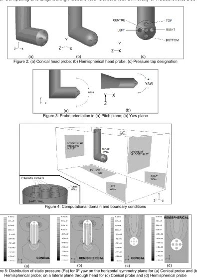
4.1 Pressure Distribution in Flow FieldFigure 5 shows distribution of static pressure around the heads of the conical and hemispherical probes at 0º yaw. Just as theoretically expected and also discussed by Morrison et al. [2], the distribution of pressure around the probe is reasonably symmetric as the probe head axis is oriented into the flow at 0º yaw and 0º pitch. The centre taps are at highest local pressure at about 700Pa for both head shapes. Whereas the peripheral taps are at significantly lower local pressures at about 350Pa.
Figure 6 and Figure 7 shows the static pressure around the probe heads for -40º and +40º yaw respectively. It is clear from Figure 6a, Figure 6b, Figure 7a and Figure 7b that the tap facing the flow for both head shapes is at a significantly higher local pressure, in the region of about 900Pa at the tip, than the opposite tap, which is at about -400Pa. This is because the tap facing the flow is at or near the stagnation pressure.
4.2 Pressure Response of Pressure Taps
A comparison of pressure response of each of the five pressure taps of both conical and hemispherical probes, as measured at the top end of each internal tube is plotted in Figure 8a through Figure 8e.
Figure 8a, Figure 8d and Figure 8e respectively show the static pressure response of the centre, top and bottom taps to variation in yaw for both conical and hemispherical head probes. Since these three taps are aligned vertically, with no variation in pitch, highest pressures for all three taps are observed when yaw is 0º and it decreases as yaw is increased in either direction. For the top and bottom taps the measured pressure drops from 18.37Pa and 14.71Pa respectively at 0º yaw to near zero values in either direction for the conical head shape and hemispherical head.
Comparison of the pressure response of the top, centre and bottom taps shows that although they show a similar trend in response to yaw. The magnitude of pressure at the centre tap is always the greatest. This is due to centre tap being located on the tip of the head.
The centre tap of the hemispherical head probe is more sensitive to yaw at -1.063Pa/º than the conical head probe at -0.611Pa/º. On the contrary the top and bottom taps of the conical head probes are more sensitive to yaw at +/-0.46Pa/º and +/-0.37Pa/º respectively than the hemispherical head probe at +/-0.3Pa/º. As discussed in Section 2, since the magnitude of error in measured pressure will not exceed the specified limits, a more sensitive response will yield a lower uncertainty in the measured pressure.
The centre, top and bottom tap pressure response also indicate that the conical head has a more symmetrical response to variation of yaw in either direction, than the hemispherical head. This makes pressure response of the conical head probe more predictable, easier to calibrate and thus more accurate.
the pressure at the right tap is expected to be highest when it is facing the flow and experiencing stagnation; this is expected to occur at or near -40º yaw. This might be due to the fluctuation of pressure at 0º yaw as observed in Figure 5b which shows a pocket of lower pressure at the tip of the right tap and pocket of high pressure further downstream inside the right tube. However this anomaly observed in the response of the right tap pressure to variation of yaw at -40º could also be attributed to the numerical error in the computational simulations due to the convergence criteria specifically for residuals of k, ε and continuity. On the contrary, the near-linear pressure response of the right tap of the conical probe follows a much expected trend.
4.3 Response of Calibration Coefficients
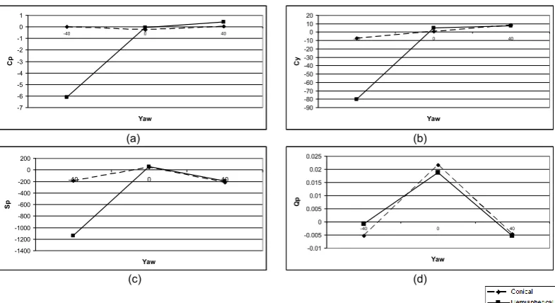
Figure 9a through Figure 9d illustrate the influence of variation in yaw to the four calibration coefficients for both the conical and the hemispherical probes.
As discussed in Section 2 the coefficient of pitch (CPITCH) is ideally expected to be more sensitive to
variations in pitch than to yaw. However Figure 9a shows that variations in yaw have a significant
influence on it for the hemispherical head probe. The response of CPITCH for the conical head probe on
the other hand shows very little variation to change in yaw. This is due to the higher level of symmetry in the pressure responses of the top, centre and bottom taps, as shown in Figure 8a, d and e. This
property of the conical head shape is advantageous over the hemispherical head, as CPITCH
dominantly influenced by variation in pitch and thus yields more accurate results.
The influence of variation in yaw on coefficient of yaw (CYAW) is illustrated in Figure 9b. It can be seen
from this figure that CYAW increases almost linearly with yaw for the conical head. However the
hemispherical head shows large variations in CYAW with respect to yaw, with a large increase between
yaw of -40º and 0º followed by a small increase from 0º to 40º. It is difficult to characterise such a response even through use of polynomial equations, especially when such a response is plotted in combination with variation in pitch, which will yield a three-dimensional surface. This property also makes the hemispherical head less favourable to the conical head. A repeat numerical simulation of the hemispherical probe at -40º yaw with smaller convergence criteria for flow residuals and a denser mesh in the vicinity of the probe could confirm the possibility of a numerical error causing the anomaly in the response of the hemispherical probe.
A similar asymmetrical change in the coefficient of total pressure (SP) for the hemispherical head is
observed in Figure 9c. The characteristic asymmetric response of these calibration coefficients in the case of the hemispherical head is attributed to the asymmetric pressure response of all the five pressure taps, which is difficult to define by equations and will consequently cause measurement errors. Whereas the conical head displays the expected symmetrical response to changes in yaw, with a maximum of 45.47 at 0º yaw decreasing to -220.17 and -191.05 at +/- 40º respectively.
The dynamic pressure at any point in the flow is representative of the magnitude of velocity at the point, and hence is an important parameter in flow metrology. The variation in coefficient of dynamic
pressure (QP) shown in Figure 9d is fairly consistent with theory [1,2] and shows variation in response
to change in yaw in either direction, symmetrically and consistently in case of both head shapes. The
conical head shape however shows a higher sensitivity of QP to variation in yaw as illustrated in Figure
9. In addition to providing ease of developing polynomial equations to characterise this response, this higher sensitivity will also translate into lower uncertainty in measured pressure as discussed in Section 2. This shows that the response of the conical head shape is easier to characterise and will provide higher accuracy in measuring flow velocity.
The response of such pneumatic probes can be studied in further detail by increasing the number of measurement points and studying their response in more detail. This may also help to identify the effective working range of both head shapes, and study the possibility of the hemispherical head being unable to measure up to +/-40º yaw due to limited range as a characteristic of the hemispherical head shape. A larger number of measurement points will also rule out any numerical errors in the CFD simulation that might occur at any point of measurement by observing the trend in responses and confirm the possibility of a numerical error for the anomaly observed for the response of the hemispherical probe at -40º yaw.
5 CONCLUSIONS
The flow field around conical head and hemispherical head pneumatic probes has been studied. The pressure responses of all pressure taps to variations in yaw have been plotted. Examination of the effect of yaw on the pressure taps in the probe head and the subsequent calibration coefficients they yield show that the conical head probe has a much more symmetrical and predictable response to changes in yaw. By contrast variations in yaw for the hemispherical head shape have a significant influence on the coefficient of pitch which shows a sensitivity of 0.15 /º for negative yaw. This adversely affects calibration coefficients, resulting in increased difficulty in developing mathematical equations to characterise the velocity vector on the basis of these calibration coefficients. Higher
sensitivity of 0.45 Pa/º and 0.35 Pa/º for the top and bottom taps respectively as well as that of QP for
the conical head shape are advantageous for accurate measurements; these characteristics far outweigh the non-linearity and asymmetric pressure response observed for the hemispherical head shape. Although more refined calibration techniques, as discussed by Morrison et al. [2] exist, the hemispherical head shape may still pose problems during calibration and consequently during the application of combination probes in flow metrology. Therefore it can be concluded that the conical head shape has many advantages over the hemispherical probe in ease of calibration and operation.
6 REFERENCES
1. Bryer, D.W. and Pankhurst, R.C. (1971). Pressure-probe methods for determining wind speed and
flow direction. London (UK): Her Majesty’s Stationary Office.
2. Morrison, G.L., Schobeiri, M.T. and Pappu, K.R. (1998). ‘Five-hole pressure probe analysis
technique’. Flow Measurement and Instrumentation. Volume 9, Part 3: pp. 153-158.
3. Dobrowolski, B., Kabacinski, M. and Pospolita, J. (2005). ‘A mathematical model of the
self-averaging Pitot tube. A mathematical model of a flow sensor’. Flow Measurement and
Instrumentation. Volume 16: pp 251-265.
4. Depolt, Th. and Koschel, W. (1991). ‘Investigation on Optimizing the Design Proces of Multi-Hole
Pressure Probes for Transonic Flow with Panel Methods’. In: IEEE, ICIASF '91 Record,
International Congress on Instrumentation in Aerospace Simulation Facilities, New York (USA), pp. 1-9. IEEE.
5. Coldrick, S., Ivey, P. and Well, R. (2003). ‘considerations for Using 3-D Pneumatic Probes in
High-Speed Axial Compressors’. Journal of Turbomachinery. Volume 125, Part 1: pp. 149-154.
6. Fluent, Inc. Gambit 2.0.4 (Geometry and mesh generation pre-processor for Fluent).
7. Fluent, Inc. Fluent 6.0.12 (flow modelling software).
8. Palmer, E., Mishra, R. and Fieldhouse, J. (2007) ‘The Manipulation of Heat Transfer
Characteristics of a Pin Vented Brake Rotor Through the Design of Rotor Geometry’ (AE14-3). In:
EAEC, 11th European Automotive Congress, May 30 – 1 June, 2007, Budapest (Hungary).
FIGURES
(a) (b)
(a) (b) (c)
Figure 2: (a) Conical head probe; (b) Hemispherical head probe; (c) Pressure tap designation
(a) (b)
Figure 3: Probe orientation in (a) Pitch plane; (b) Yaw plane
Figure 4: Computational domain and boundary conditions
[image:8.595.120.516.44.600.2](a) (b) (c) (d)
Figure 5: Distribution of static pressure (Pa) for 0º yaw on the horizontal symmetry plane for (a) Conical probe and (b) Hemispherical probe; on a lateral plane through head for (c) Conical probe and (d) Hemispherical probe
[image:8.595.96.529.611.706.2](a) (b) (c) (d)
Figure 6: Distribution of static pressure (Pa) for -40º yaw on the horizontal symmetry plane for (a) Conicalprobe and (b) Hemispherical probe; on a lateral plane through head for (c) Conical probe and (d) Hemispherical probe
CONICAL CONICAL
CONICAL
CONICAL HEMISPHERICAL
HEMISPHERICAL
HEMISPHERICAL
(a) (b) (c) (d)
Figure 7: Distribution of static pressure (Pa) for +40º yaw on the horizontal symmetry plane for (a) Conical probe and (b) Hemispherical probe; on a lateral plane through head for (c) Conical probe and (d) Hemispherical probe
0.000 5.000 10.000 15.000 20.000 25.000 30.000 35.000 40.000 45.000 50.000
-40 0 40
Yaw C e n tr e T a p P re s s u re ( P a ) (a) -5.000 0.000 5.000 10.000 15.000 20.000 25.000 30.000
-40 0 40
Yaw L e ft T a p P re s s u re ( P a ) (b) -10.000 0.000 10.000 20.000 30.000 40.000 50.000 60.000 70.000 80.000 90.000
-40 0 40
Yaw R ig h t T a p P re s s u re ( P a ) (c) -5.000 0.000 5.000 10.000 15.000 20.000
-40 0 40
Yaw T o p T a p P re s s u re ( P a ) (d) -2.000 0.000 2.000 4.000 6.000 8.000 10.000 12.000 14.000 16.000
-40 0 40
[image:9.595.115.512.181.475.2]Yaw B o tt o m T a p P re s s u re ( P a ) (e)
Figure 8: Comparison of pressures (Pa) for both head shapes measured at (a) Centre tap, (b) Left tap, (c) Right tap, (d) Top tap, and (e) Bottom tap.
-7 -6 -5 -4 -3 -2 -1 0 1
-40 0 40
Yaw Cp (a) -90 -80 -70 -60 -50 -40 -30 -20 -10 0 10 20
-40 0 40
Yaw Cy (b) -1400 -1200 -1000 -800 -600 -400 -200 0 200
-40 0 40
Yaw Sp (c) -0.01 -0.005 0 0.005 0.01 0.015 0.02 0.025
-40 0 40
Yaw
Qp
(d)
Figure 9: Comparison of calibration coefficients for both head shapes. (a) CPITCH, (b) CYAW, (c) SP, and (d) QP.
HEMISPHERICAL
HEMISPHERICAL
CONICAL
[image:9.595.116.509.509.723.2]