Thesis by
Jai Sam Kim
In Partial Fulfillment of the Requirements
for the Degree of
Doctor of Philosophy
California Institute of Technology
Pasadena, California
1982
ACKNOWLEDGEMENTS
It is a pleasure to acknowledge and thank my adviser, Professor Murray Gell-Mann, for his patience and guidance throughout the course of my graduate school program. His comments and suggestions were useful and most of all inspirational.
1 wish to thank the general graduate advisor, Professor Frautschi, for babysitting me when Professor Gell-Mann could not take care of me due to late Margaret's illness and many helpful discussions. I am also grateful to Professor Politzer and Dr. Ambjorn for helpful discussions. Conversations with Professor Patera and Dr. Slansky were also valuable.
I am very grateful to Dr. S.H. Lee of Chevron Oil Co. for helping me to write fortran programs. I am also grateful to Dr. R. Howard of the Cal Tech mathemat-ics department for valuable discus~ions on differential geometry, I wish to thank Richard Brenner, Eugene Brooks, and Drs. Richard Hughes, Rajan Gupta, Stuart Stampke, and John Valainis for collective wisdom. I wish to thank Helen Tuck for encouraging me in hard times.
ABSTRACT
TABLE OF CONTENTS
CHAPTER I
l.1 INTRODUCTION 1
l.2 HIGGS PROBLEM AND ORBIT PARAMETERS 6
CHAPTER II ONE IRREDUCIBLE REPRESENTATION
II. l OUTLOOK WITH AN EVEN DEGREE HIGGS POTENTIAL 9
II.2 GENERAL FORMALISM 16
Il.3 THE GENERAL STRUCTURE OF THE ORBIT SPACE OF
ONE IRREDUCIBLE REPRESENTATION 26
II.4 APPLICATION TO SU(N) ADJOINT REPRESENTATION 30
CHAPTER III TWO IRREDUCIBLE REPRESENTATIONS
III.1 GENERAL FORMALISM 39
III.2 THE GENERAL STRUCTURE OF THE ORBIT SPACE OF
TWO IRREDUCIBLE REPRESENTATIONS 47
lll.3 APPLICATION TO SU(N) ADJOINT+ VECTOR REPRESENTATIONS 50
CHAPTER IV COMPLETE ORBIT SPACES
IV. l COMPLETE ORBIT SPACES OF ADJOINT REPRESENTATIONS 104
N.2 TWO IRREDUCIBLE REPRESENTATIONS 144
CHAPTERV GENERALIZATION TO NON-LINEAR POTENTIAL 152
LlST OF FIGURES AND TABLES
Fig . .II.1.1
Fig .. II.1.2
Fig .. II.1.3
Fig .. II.1.4
Fig .. II.2.1
Fig .. Il.2.2
Fig .. II.2.3
Fig . .II.2.4
Fig .. Il.4.1
Fig .. II.4.2
Fig .. III.1.1
Fig . .III.1. 2
Directional behavior of a Higgs potential for one irrep 10
Moving directional minima 10
The k-line for an even degree Higgs potential touching a two-dimensional orbit space
The k-surface for an even degree Higgs potential touches a three-dimensional orbit space
Movement of the k-contour for the case A. A1, B, m2
>
0 Typical appearance of the k-contour for each sign of A1 and BIn the m 2
<
0 case, the directional behavior of the potential evolves 1213
18
20
as the k-contour pivots 22
Movement of the k-contour for the cas·e A. A1, B, -m2
>
0 23 The (projected) orbit space of SU5 adjoint 33The (projected) orbit space of SUN adjoint 38
Directional behavior of a Higgs potential for two irreps 40
The k-cone for an even degree Higgs potential for two irreps touch-ing a three-dimensional orbit space
Fig .. III.3.1 The boundaries of the orbit space for SU5 adjoint +vector
45
53
57 Fig .. III.3.2 The strata of SU3x U1 and SU2xSU2x U1
Fig .. III.3.3 The stratum of SU3
Fig .. III.3.4 Random stratum points for SU5 adjoint+ vector
Fig .. III. 3. 5 Evolution of the k-parabola
58
60
Fig .. III.3. 6 The k-cone successively intersecting the plane ?'= 0 66 Fig .. III. 3. 7
Fig .. III.3.8 Fig .. III.3. 9
The allowed region for directional minima of solution IV 67
The k-parabola sweeping the orbit space 71
The little group of the absolute minimum for each sign
combina-tions of A1 and B1 (the SU5 case) 72
Table.IIl.3.1 Turning points of the curves in Fig. III.3.10 78 Fig .. III.3.10 The orbit spaces of SUN adjoint+ vector 80 Fig .. I1l.3. ll The little group of the absolute minimum for each sign
combina-tions of A1 and B1 (the SUN case) 81
Fig .. III.3.12 The indented segments of the orbit space boundary cannot yield the absolute minimum
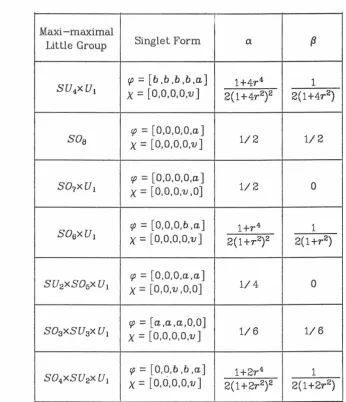
Table .lII.4-.1 Maxi-maximal little groups of 8010 adjoint + vector Fig . .III.4.1 The orbit space of 8010 adjoint +vector
Table.III.4.2 Maxi-maximal little groups of S02n adjoint + vector yielding the absolute minimum
Table.III.4.3 Maxi-maximal little groups of 807 adjoint+ vector Fig .. III.4.2 The orbit space of S07 adjoint +vector
Table.III.4.4 Maxi-maximal little groups of S02n+I adjoint + vector yielding the 82 90 91
92
97 98absolute minimum 99
Table.IV.1.1 List of Casimir invariants of classical and exceptional groups 106 Fig .. IV.1.1 The complete orbit space of SU4 adjoint
Fig .. N.1.2 The complete orbit space of S07 adjoint
Fig .. IV.1.3 The complete orbit space of ~p6 adjoint
Fig .. IV.1.4 The complete orbit space of SU5 adjoint
Fig .. IV.1.5 The complete orbit space of S09 adjoint
Fig . .IV.1.6 The complete orbit space of
B_p
8 adjointFig .. IV.1. 7 The complete orbit space of S08 adjoint Fig . .IV.1.8 The complete orbit space of F4 adjoint
Vig .. IV.1.9 The complelc orbit space of Oh vector
Fig . .IV. l.10 The complete orbit space of S05 symmetric tensor
Fig ..
IV.2.1Fig . .IV.2.2 Fig .. V.1.1
Fig .. V.2.1
The complete orbit space of SU3 adjoint
+
vectorThe complete orbit space of S05 adjoint + vector
A curve defined by eq. (V.1.8) passes through an orbit space
A cone defined by eq. (V.2.6) passes through an orbit space
115
119
124
129
133
140
141
142
146
149
154
1.1 INTRODUCTION
After the discovery of the Higgs mechanism [1], it has been employed
almost exclusively in the gauge symmetry breaking problem because it breaks a
local gauge symmetry without damaging the renormalizability [2]. Though it is
not the only known mechanism to do such a job [3,4], certainly it is the only
tractable one. Partly due to its tractability it drew considerable attention of
theoretical physicists despite some ugly features. There is a consensus that
though it may not be a fundamental mechanism it would describe the effective
phenomena arising from some unknown fundamental interactions. It was
applied to the unification of electromagnetic and weak interactions [5] with
great success and subsequently to fancier grand unification theories [6]. Here
some major difficulties arose, namely the gauge hierarchy problem [7] and
prol-iferation of Higgs parameters etc. As the spontaneous symmetry breaking
mechanism was devised by Landau [8] to explain the second order phase
transi-tion in type II superconductors, the mechanism has been widely employed in
condensed matter physics [9, 10]. The importance of the Higgs problem in the
contemporary theoretical physics is indicated by the existence of several
exten-sive review articles [ 11].
The technical problem of minimizing the Higgs potential and finding the
symmetry of the vacuum actually was overlooked by most model builders. It is
not the least aspect of model building because the representation content of
scalar particles is not the only ingredient in determining the vacuum symmetry;
the actual structure of the potential also comes in to play a major role.
from branching rules of the Higgs representation.
It seems a bit in reverse order to review historical developments of the theory before presenting some explanations of the terminology. We urge the reader unfamiliar with the subject to skip the following paragraph for a moment until he finishes reading the whole of chapter I.
There are three major mathematical results one needs to solve the Higgs problem:
1) invariant polynomials specify orbit;
2) there is a basic set of invariant polynomials; 3) the structure of the orbit space.
The first result which is the most important for our purpose was clearly per-ceived by Aronhold [12] in 1863. The second result is due to Hilbert [13]. As Weyl stated in his book [ 14], "Hilbert founded the proof of the invariant theoretical
main theorems on a general proposition concerning polynomial ideals that is one of the simplest and most important in the whole of algebra". Relatively recently much work was done [15] on the orbit space structure of a single irreducible representation. These results lay in the backyard until very recently. Brout [ 16] first noticed the importance of the orbit structure and of
the conjugacy classes of subgroups. Michel and Radicati [ 17, 18] took further steps in this direction and in addition studied the geometrical structure (in the
field component space) of orbits. They defined the orbit parameters and expli-citly constructed the orbit space. Based on a theorem by Michel [ 17]
concern-ing the critical orbits, they conjectured that a fourth degree Higgs potential preserves the maximal symmetries possible. Later Li [ 19] simplified a set of Higgs fields by group transformations, which was equivalent to parametrizing
while keeping the magnitudes of the Higgs fields constant instead of extremizing the whole potential with respect to field components, which was partly in confor-mity with Michel's method but was a first step towards new methods of minimi-zation. Subsequently Gell-Mann and Slansky [22] attempted to generalize
Michel's conjecture for one irreducible representation to two irreducible
represenlalions. Most recently Abud and Sartori [23] fully utilized the above results in their work and treated each invariant as a coordinate in a hyper-space where an orbit is represented by a point. They further unveiled some geometri-cal aspects of the hyper-space.
The geometrical method that is going to be reviewed in this thesis, is based on a collection of papers [24,25,26,27] published by the author plus work presently in progress [28]. Although this method was inspired by Prof.
Gell-Mann's remark in his lecture concerning the existence of some parameter speci-fying the orbit of SU3 adjoint representation, it carries the foregoing works further and elucidates the rich geometrical nature of the extremization prob-lem. It is based on the observation that the orbits and the conjugacy classes of subgroups are the relevant quantities to describe the minimum of the Higgs
potential which is invariant under a linear transformation of a compact Lie group on the scalar fields. Hilbert proved that there is a basic set of invariants
such that all the other invariants are expressed in terms of them and provided a systematic method to find all the basic invariants. It has been known that
invari-ants specify orbits, i.e., one can view an orbit as a point in a (l
+
1)-dimensional vector space. How can we describe a direction in such a space? Indeed there is aregion (called the orbit space) in the orbit parameter space, which can be
regarded as al-dimensional vector space.
Since the scalar potential is a group invariant function it can be e1..rpressed
in terms of the basic invariants. But a classical scalar potential is restricted to
be a fourth degree polynomial of the scalar fields due to renormalizability*.
Because of this restriction it is normal that a subset of all the basic invariants
appear linearly in the Higgs potential. The potential can be written in terms of
the norm of the field and a few orbit parameters. For a given set of orbit
param-eters we can survey the behavior, particularly e:Ktrema, of the potential along
the corresponding direction in the vector space. By varying the orbit
parame-ters we can survey the whole space in search of the absolute minimum where
the vacuum resides. Because of the linearity the absolute minimum of the potential occurs on the boundary of the orbit space, which is a projection of the
complete orbit space.
The potential can be minimized abstractly for a general representation of a
general compact group. The difficult part of extremizing the potential in the
conventional methods is equivalent to finding the orbit space boundary, which is
unique for each different representation. In our original works we used the
Michel-Radicati conjecture for one irreducible representation (irrep) and the
Gell-Mann-Slansky conjecture for two irreps as a guide to find the orbit space
boundary. Later we found that much work has been done by mathematicians
[ 15] on the structure of the orbit space for one irrep. Their results were derived
without referring to invariants at all and, though general, are not too
under-standable for an average physicist. With our formalism many things become
intuitively clear. The main result is that the orbit space consists of some
dimensional volume occupied by the generic stratum of the lowest level
sym-metry group and all the other strata of higher symmetries forming the singular
boundaries. The strata of the highest symmetries are the most singular.
As we shall see the absolute minimum of the Higgs potential occurs on the
most protrudent portions of the projected orbit space boundary. Though there
is no coherent logical relationship between singularity and protrusion of a
stra-tum, we observe that most singular strata are normally most protrudent (at
least locally though not globally). Consequently the absolute minimum of the
potential is most likely to occur at the stratum of highest symmetries in
1.2 HIGGS PROBLEM AND ORBIT PARAMETERS
Though our method can be applied to any kind of Higgs potential. we
will take a rather simple case to show the main ideas. In a non-abelian gauge
theory, where the scalar potential has a symmetry G x reflection and the
scalars transform as an n-dimensional irreducible representation
H.
of G*, theHiggs potential can be written as
1 n 1 n
V(cp) = - - m2
l;
So/Soi+
- A ( ~c;otc;oi )
2+
2 i=l 4 i =1
(I.2.1)
V( cp) is invariant under a group transformation
where T('IJ) is an n-dimensional matrix corresponding to a group element. In
general
N
T('IJ.) = exp(-i~ 'IJLXL) ,
i=l
where XL are generators of the group and 'IJL are group parameters specifying
an element of the group.
As is well known, due to the negative mass term the minimum of the
poten-tial occurs at some nonzero values v of cp. The vacuum, defined to be at the
minimum of the potential. respects only a subgroup G' of the symmetry group G
of the Lagrangian. Mathematically speaking, T('!J) v = v only if T('IJ) is an
ele-ment of G' c G, otherwise T('IJ.) v '/: v.
When one tries to find the minimum of the potential, one faces significant
difficulties;
1) Finding the solution for arbitrary coupling coefficients by setting
al' I acpi = 0 is very difficult because it requires us to solve simultaneous cubic
equations of too many unknowns.
2) For numerically given values of the coefficients we may try to use some
well-developed computer programs to minimize the potential. But it will not be
helpful because the minimum occurs along valleys in cp space. To put it more
clearly, we may choose rp1 = v and ~X1.X2.X3~ as our subgroup singlet and
gen-erators respectively, or we may equally well choose rp2 = v and ~X4.X5.X6~. In
general there is a continuum of equivalent sets of C,Oi and ~XL .XM .XN
J.
The Higgspotential is totally blind to such differences.
We will now introduce some useful group theoretical concepts. The orbit of
C,Oa is defined to be the set of states rp(a) that can be expressed as rp(a)
=
T(iJ) C,OawiLh '/'( 19) un clement of G. The little group of Y'a is defined to be the subgroup G'a of G that leaves C,Oa invariant, T(iJ)cpa,
=
cpa, for T(iJ)EG'ac
G. Consideringthat T('l'J)cpa = T(Oc,oa is true if and only if T('l'J)
=
T(0T(1'J') with T('l'J') anele-ment of G'a we see that the states of an orbit are in one-to-one correspondence
with the coset GI G'a· It can easily be shown that the little group G'b of any
state rp0 on the orbit of C,Oa is conjugate to G'a.· If the T('l'J) are unitary then all
the states rp(a) have the same norm c,o;c,oa. In general. there is a continuum of
dis-tinct orbits respecting the same little group up to conjugation. The set of all
such orbits is called the stratum of the little group. Note that if the little groups
of two orbits are distinct then the orbits are distinct. However the converse is
not true, i.e., if two orbits are distinct their little groups are not nec~ssarily
Two important theorems concerning invariants and orbits can be found in the literature:
Theorem 1; Invariant polynomials P(cp) specify orbits of cp.
From this theorem [ 12] we see that each invariant polynomial in the Higgs potential is conslant on an orbit and thus is a function of orbits. When we seek a solution to the Higgs problem, we are actually seeking the orbit that minimizes the potential, and its little group.
Theorem 2; There exists a set of invariant polynomials Ia(cp), called the
integrity basis such that every invariant polynomial P(cp) can be expressed
as a polynomial of Ia. : P(cp) = P[Ia(cp)] .
This is the celebrated theorem of Hilbert's [ 13]. The invariants in the integrity basis are not necessarily independent and indeed for some representations there are constraints among them. We will call the complete set of independent invariants, basic invariants. The number (l + 1) of basic invariants is different for each different representation
.H.
Thus we can visualize an orbit as a point in the (l+l)-dimensional space of Ia·Our crucial observation is that the dimensionless ratios of invariants to the magnitude of the cp vector, for example
(I.2.2)
can also be used to specify strata, and yield a powerful tool in minimum prob-lem. We will call the dimensionless ratios orbit parameters. They can be con-sidered as a set of generalized angles containing all the directional information. From the definition we can readily see that their ranges are bounded and thus they occupy a localized region (called the orbit §pace)* in the orbit parameter space, which can be regarded as al-dimensional vector space.
CHAPTER II ONE IRREDUCIBLE REPRESENTATION
Il.
l
OUTLOOK WITH AN EVEN DEGREE HIGGS POTENTIALBefore we analyze the general scalar potential let us consider a simple case
to develop general ideas. Suppose the scalar fields transform as an n-dimensional irreducible representation (irrep) R of a compact (or finite) group G and in addition have a reflection symmetry. Then the most general Higgs potential can be written as
where
Since we want the potential V( cp) to increase to
+
00 as 11cp11400 , we impose a condition on the coupling coefficients;(IJ.1.2)
Our new variables are 11cp11 and Ai (s;?). Since the potential is made of quadratic and quartic invariants only, normally A,;. do not constitute the complete set of orbit parameters. However we shall soon see that these constitute the complete set of 1 ,!'umeters needed to specify the absolute minimum of the potential.
this direction;
V
= -
~
m2IIY'11+
!
A' 11Y'112 , (Il.1. 3)where m and A' are constant numbers. This function behaves like Fig. II.1.1. The extremum for this particular choice of ~ (~) is found by setting
(II.1.4)
equal to zero. We obtain
(Il.1.5)
which is automatically positive for m2
>
0 due to the condition (II.1.2). Noting that(II.1.6)
is always positive due to the condition (II.1.2), we see that eq.(II.1.5) is a local
minimum (which we call the dfrectianal minimum of the potential in the direc-tion of Y' specified by Ai(~).
v
v
At the directional minimum
'Va(So) = V(So)J11~ll=ll~ll
0
_ 1 m4
- - 4
(A+
A1tq+ AzA2+ · · · ) (II. 1. 7)As we change the direction in So space (i.e., the t..i(~)), the location of the
minimum will move around as in Fig. II.1.2. To find the absolute minimum we just have to look for the lowest of those directional minima. Since
av
a~ (II.1.8)
V is a monotonic function of Ai. Thus the absolute minimum of V is not at
a
VI a~ = 0, but at the boundary points of the region of "physical" ~.To find these boundary points, note that the orbit parameters are dimen-sionless ratios of invariants such as eq.(I.2.2), i.e., they depend on~ whose
mag-nitudes are less than one. These defining equations permit a precise determina-tion of the region of "physical"
t..i.
In particular it is immediately clear that forany configuration of '(/;, the range of
t..i
is bounded above and below:In an actual calculation the first practical task will be to calculate the physical region of Ai('(/;), which we shall call the orbit space*.
•A proper description is the stratum space, which is a projection of the true orbit space. Th~
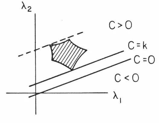
Suppose there are two orbit parameters Ai and f..2 . In the /..i - f..2 plane, the
orbit space will look like the warped polygon in Fig. II.1.3. It is important to note
(viz, eq. (I. 2. 2)) that the orbit space is independent of Higgs coupling coefficients
and masses, though it does depend on the group and the representation.
Turning our attention to the potential, let us put
(II. l. 9)
Jl'or given values of A, A1, A2 and C, this will represent a line in Ai - f..2 space (Fig.
II.1.3) According to condition (II.1.2) the line can only intersect orbit space when
C
.
>
0. As we increase C at fixed A, Ai, A2 , the line will sweep the orbit space.The minimum physical value of C will occur where the line first touches the orbit
space. By eq. (II.1. 6) this corresponds to the absolute minimum of the Higgs
potential. Above the absolute minimum of V there is a continuous range of V and
11'fJ110 where
a
VIa
11'fJ11=
0 can be satisfied by some choice of f..i. As we furtherincrease C, the line finally leaves the orbit space at the highest of the
direc-tional minima where V has the form of the upper curve in Fig. II.1.2.
C>O
[image:21.613.183.447.483.687.2]Our considerations with Fig. II.1.2 have suggested that V has no other extremum than the absolute minimum and the local maximum at 11cp11 = 0.
For some special values of A1 and A2 the line can first touch the boundary of orbit space at two points. In such cases there are two different valleys of extrema (two orbits) that cannot be connected by a gauge transformation and the vacuum has an accidental degeneracy.
If there are more than two orbit parameters, then
(II.1.10)
represents a plane in f.. space and the situation can be depicted as in Fig. 11.1.4. The procedure to find the minimum will be the same as before. Since the abso-lute minimum always occurs at the boundary of the orbit space, we have to find the (s-1) surface parameters and the value of the potential at the first contact point in the s-dimensional orbit parameter space. However the orbit space of a single irrep is normally conjectured to be star-shaped (Fig. II.1.4) and normally all we need to know is the location of the cusps. Detailed e~rplanation will be presenled i.n Cll 11.2-3 and CHV.
When the representation is complex, the potential can in general contain
terms of the type
( H ~jktCfJiCfJjCfJkCfJt+ complex conjugate)
= 2
JHI
cos[h+
'6(~)] 17(~)1ISol12 , (Il.1.11)where
I
HI =
magnitude of H ,h
=
argument of H ,At the minimum of the potential, h
+
1J = 1f, and 11(~) is determined in the sameway as the Ai.
In problems where cubic potentials or effective potentials are considered,
the potential takes the general form
V(cp)
=~Al
ISol
I+~
[B1f11(~)
+
B2f32(~)
+ ... ]I
I
cpl 1312+
!
[
c
+
ca
1 (~)
+
...
J
I 1 cpI 1
2+
~
[
n
io
i (~)
+ ... ]
I I
cpI I
512+
· ·
·
(IL i.12)If we choose a direction in cp space, all the orbit parameters will become con
-stant numbers and we can easily see how the function behaves in that direction
of cp. However due to Theorem 2, some orbit parameters associated with higher
degree (~5) polynomial invariants are polynomials of lower degree parameters.
Eventually the problem will become non-linear and one may expect that detailed
solution will be far more complicated. However, as we shall see in ClN the
Il.2 GENERALFORMAIJSM
Let us start with a case where there is one cubic invariant polynomial and one non-trivial quartic invariant polynomial. As we will see our result can be trivially extended to a more general case where there are more cubic and quar-tic invariant polynomials.
To simplify the notation, we set
r
=
I
I
c;
I I
112 , (II.2.la)(ll.2.lb)
B'
=
B{3 . (II.2.lc)Then the Higgs potential takes the form,
m2 B' A'
V= - - - r2
+
- r3+
- r42 3 4 (II.2.2)
We impose the positivity condition,
(II.2.3)
on Lhe coupling coefficients in order to ensure that V4+00 as
11c;114
00 •As eA.rplained in the previous section, since the potential is a monotonic function of a and (3 we do not differentiate with respect to a and (3 to find the e}...1.remum of the potential. Differentiating with respect to r we obtain,
av
or = r (-m2+
B'r+
A'r2) . (Il.2.4)
There are three extrema:
(ii)
(iii) r 0 =
-B'+
V
B'2+
4A'm22A'
-B'-
V
B'2+
4A'm2 2A'(II.2.5b)
(II.2.5c)
To find out the nature of each extremum, let us check the second derivative,
a
2v
- - = -m2
+
2B'r+
3A'r2ar
2The value of the second derivative at each extremum is:
(i)
(ii)
(iii)
-m2
VJ5
(05 - B') 2A'VJ5
(...JJJ+
B') 2A'where D
=
B'2+
4A'm2.(II.2.6)
(II.2. ?a)
(II.2.7b)
(II.2.7c)
In order to prevent confusion, we will treat the three cases, m 2
> 0, m
2= 0, and m 2< 0, separately.
(a) m2
>
0In this case, taking eq. (Il.2.3) into account, D is automatically positive and greater than
I
B'I
. Checking signs in eqs. (Il.2.5) and (II.2.7) we find that solution
(i) is a local maximum. solution (iii) is unphysical, and solution (ii) is a local
minimum for either sign of B'. The local minimum is lower when B'< 0. Substituting solution (ii) into eq. (II.2.2) we obtain
m4 m2B'2 m2B' B'3 -B'+ VB'2
+
4A'm2Va
= - -4-A-' - 12A'2 + ( 3A' + 12A'2H
2A'~
= -
!£_which is negative definite for A'> 0, m2
>
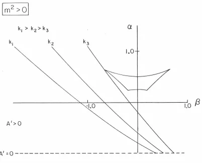
0, and B'< 0. This equation defines acurve in the r.x-{3 plane (or A'-B' plane). To get a rough idea, we have made
com-puter generated plots of the contours for several k values for a particular case
(A, A1, B, m 2
>
0) (Fig. II.2.1). Despite the complicated look of eq. (II.2.8), thecontours turned out to have simple shapes. For a given k, the contour is a
smooth curve with no extrema in the region A
+
A1r.x>
0. Each k contour passesthrough the point [ ex= (m 4
/ k -A)/ A1, {3=0] to reach the point
[ r.x=-A/ A1, {3=.J213m3/-.JkB] where A' goes negative. Ask is reduced from
+
00, where the contour is the horizontal line cx=-A/ A1, the k contour rises up
and slides to the right in the case (A, A1, B, m2
>
0). When it makes the firstcontact with orbit space, it yields the absolute minimum of the potential. As k is
further reduced, the k contour sweeps through the entire orbit space.
a
1.0
A'>O
A'
=
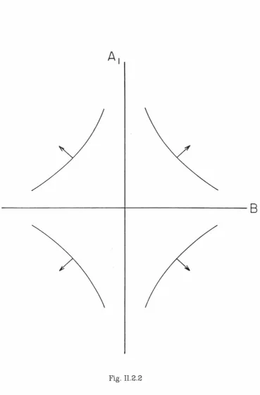
0 [image:27.612.117.519.373.697.2]The above statements on the movement of the k contow~ are justified by
checking the direction of the gradient vector Vk
=
(Bk I arx, ak I 8{3). In terms ofp
=
v
B'2+
4A'm2/IE'
I
>
1, its components are:1 Bk 1 Bk
- 4aA'
= - 4A1arx
=
m 4 ( p+
1 ~2>
0 , 4A'2 p - 1= m2
IB'I
m2 B'2IB'I
+VB'
2+
4A'm2 6A'2+ (
3A'+
4A'2 )( 2A' JIB'I
1+
---;:::~::=:====;:;--+
m2IB'I
IB'l
3VB'
2+4A'm2( 3A'
+
12A'2H
2A'1
:: m2
I
B'I
(p+
1)2>
0 6A'2 (p - 1)(Il.2.9)
(Il.2.10)
The orientation and direction of movement of the k contour as k decreases are
Using eqs. (II.2.9) and (II.2.10) one can compute the second derivative:
d2A' __ .!!.-__(Bk/ BB')
dB'2 - dB' (ak; aA')
=
14 (p-1) 2>
0 .9m p (II.2.11)
One finds that the k contour is always concave in the direction towards which it is moving.
(b) m2
=
0Though the potential has a simplified structure in this case, it still has directional extrema. Solution (i) is an inflection point and solution (ii) with
B'< 0 is the directional minimum.
Eq. (Il.2.8) reads, for m2
=
0 and B'< 0, as follows:IB'l
4Vo
= - 12A'3k
4
which is negative definite. Solving eq. (II.2.12) for A' we obtain
A' =
I
B' 1413; (3k )113 .(II.2.12)
(II.2.13)
This is a familiar curve, somewhere bclwecn a slraighl line and a parabola, and
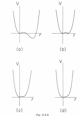
(c) m2
<
0In the region where B'2
- 4A'
I
m2 J > 0, solution (i) is a local minimum,solu-tion (ii) with B'
<
0 is a local minimum, and solution (iii) with B'<
0 is a local maximum. If the cubic term is strong enough, solution (ii) will be the lower minimum. Otherwise solution (i) will be the lower. In the region where B'2- 4A'Im
2I
<
0, there is only one local minimum at the origin.Directional behavior of the potential is most complicated in this case. The evolution of the potential through the configurations listed above as k decreases is shown in Fig. II.2.3.
v
v
r
(a)
( b)
v
v
r
r
(c)
( d)
[image:31.613.148.453.283.727.2]I
m2<ol
a
8'2
k
=0
'- 2
A
-9lm
2
1
\
8'2
m4k1>k2>k3
A'=
41 m
21k = - 3A'
k3
k,
k2
A'> 0
A'
=O
- - - - -
-
- -- - -
- - - , - [image:32.613.115.548.174.530.2]Eq. (II.2.8) reads, for m2
<
0, and B'< 0, as follows:= _
m4 + lm2l IB'l2 + lm2l IB'IVa
'1A' 12A'2 ( 3A'IB'l3, IB'l+v'B'2-4A'lm21
~(
2A' J4
12A'0-p2)2 (3p4 + 8p3 + 6p2 - 1),
k
4 (II.2.14)
which is not negative definite for 0 ~ p ~ 1. Eqs. (II.2.9), (II.2.10), and (II.2.11)
can be used for the m2
<
0 case withm2 replaced by-jm21 and (p-1) by (1-p).The direction of the gradient vector Vk =(ak; aa, ak; a{3) is the same as before.
The k contour is again concave. The k contour does not slide but pivots about
the point (a=-A/ A1, (3=0). For simplicity let us concentrate on the case
A, A1, B, - m 2
>
0 (Fig. II.2.4). As k is reduced from +00 the k contour pivotsclockwise until it meets the orbit space. As k is reduced to zero, which happens
whenp = 1/ 3, the contour becomes the parabola,
2 B'2
A'=
g
jm21 . (II.2.15)Beyond this point k takes on negative values. As the k contour touches and
becomes identical to the parabola B'2- 4A'lm2
1=0
at k= -
m4/3A', the twoextrema at r0 ~O coincide and become an inflection point leaving the origin as
the only extremum, the absolute minimum.
lf the first contact occurs with the k =O contour an interesting phenomenon
occurs. In this case we have a spontaneous symmetry breaking at T0 ~O and no
symmetry breaking at T0 =O (Fig. II.2.3b). It will be interesting to see what kind
11.3 THE GENERAL STRUCTURE OF THE ORBIT SPACE OF ONE IRREDUCIBLE
REPIU!SENTATION
Due to the monotonicity of the Higgs potential with respect to the orbit parameters the absolute minimum occurs on the boundary of orbit space, at the point of first contact with the potential minimizing k-surface. If the k-surface is
ftat (CHII.1) or concave in the direction towards which it is moving (CHII.2), its
point of contact is further restricted to non-concave segments on the orbit space boundary. These features are universal to a general Higgs potential for scalar bosons belonging to an irreducible representation of the symmetry group. What is different for each different representation is that each has its own unique orbit space.
Although the structure of the orbit space for an irrep was unveiled [ 15] abstractly by a group of mathematicians, we derived the same result in a more intuitive way. An important clue leading to a general description of an orbit
space is found in Michel's work. Michel and Radicati [ 17, 18] were among the first
who realized the importance of the orbit structure and of the conjugacy classes of subgroups. They took further steps in this direction and in addition studied the geometrical structure (in the field component space) of orbits. They conjec-tured that if the representation of the symmetry group G of a fourth degree Higgs potential is irreducible on the real, its minima preserve ma:h.imal little groups. This was based on a theorem by Michel [ 17] that when 11cp11 is held con-stant, all invariant polynomials are stationary at a critical orbit, which is
iso-lated in its stratum and has a maximal little group. This theorem amounts to
saying that there is a cusp at each critical orbit point. If these cusps are the
only non-concave portions of the boundary, the Michel-Radicati conjecture is proved. These considerations led us to anticipate that the orbit space of one
Let us give somewhat more specific arguments on the structure of a com-plete orbit space of one irrep. First the dimension of a comcom-plete orbit space for one irrep is one less than the number of independent invariant polynomials. The latter number is equal to the number of simplified Higgs field components, which we have called CfJi so far. The two sets of parameters are equivalent ways of specifying a stratum point. The non-linear transformation rules among them are given by the definitions of the orbit parameters. Let us denote the ratios of the components as before, ri
=
cpd
CfJt+I· If we consider the Jacobian determinant B(a1, a2. · · · .at) I a(r 1, r2 , · · · .rt). then we can easily deduce the necessary condilions for a boundary poinl:At a point on the bo'undary point of the orbit space' the rank of the
Jacobian determinant is less than or equal to (l-1).
When the rank of the determinant is (l-s) in some regions of the orbit space, the regions form (l-s )-dimensional surfaces. The regions are singular regions embedded in higher-dimensional space. Let us define
P
= (a1i a2 , · · · , at) to describe the boundary conditions in more detail. When s =l in some regions they correspond to singular points, i.e., cusps. Equations for them are(II.3.1)
When s =(l -1) in some regions they correspond to singular curves, i.e., edge curves. Equations for them are
(II.3.2)
(II.3.3)
where ~ij(aaal ari)(aab/ ari) = 0 is allowed for some (a,b) but not for all.
Eq. (JI.3.1) imposes l conditions on l ri 's, implying that the stratum of the cusp has only one parameter, i.e., one singlet. This guarantees that the little group of the cusp is a maximal little group. Eq. (II.3.2) imposes (l -1) conditions
on l ri 's, leaving two parameters. The stratum of the curve has a semi-maximal* (or maximal) little group. Eq. (II.3.3) imposes (l-2) conditions on l ri 's, leaving
three parameters. The corresponding stratum commonly has a one-level lower little group.
From the above considerations and some examples (CHII.4, CHIV. l) we can picturize the complete orbit s·~ ... ..;e of one irrep as follows; On the boundary of the complete orbit space there are cusps of maximal little groups, singular curves of semi-maximal little groups connecting the cusps, and singular sur-faces of lower level little groups stretching between the curves, and so on. Inside the boundary all the points belong to a stratum, called the generic stratum, corresponding to a unique little group. It is noteworthy that the lower level little groups are subgroups of higher level little groups when the strata of the latter lie on the strata of the former. For example, when a cusp lies on two curves of
different little groups they are subgroups of the little group of the cusp.
The main result of ref. [ 15] is that the generic stratum occupies some l-dimensional volume (an open, dense, and topologically connected region) and all
the other lower dimensional strata form the singular boundaries of the generic stratum. It is noteworthy that this pattern repeats whichever stratum we start
from. For example, if we start from a two-dimensional surface the curves close most of the boundary of the surface and the cusps close both the curves and the surface.
If the Michel-Radicati conjecture is to hold, the projected orbit space
(con-structed out of the invariants employed in the 4th degree Higgs potential) must have further properties; Cusps should be globally most protrudent. In other words, all the boundary surfaces must lie inside the polyhedron which is con-structed by drawing straight lines between all the cusps. AB we shall see in CHIV. l, the complete orbit spaces do not have this property. Whether or not the projected orbit spaces have the property remains to be seen.
II.4 APPLICATION TO SU(N) ADJOIN1' REPRESENTATION
II.4.1 THE IDGGS POTENTIAL FOR SU(5) ADJOINT REPRESENTATION
In the spirit of doing simple things first and then extending to a general case we will first consider SU5 adjoint [30] to show concretely how our method is
applied. We will consider the most general Higgs potential invariant under SU5 gauge transformation:
(II.4.1)
Diagonalizing the traceless hermitian matrix cpi i, we obtain
m2 o B 5 A 5 A1 5 V( So) = - -
I:
Sof
+
-
2:
~(+ - (
I;
cpi2 )2+ -
I;
cp{2 i=l 3 i=l 4 i=l 4 i=l
(II.4. 2)
with
(II.4.3)
We further express the potential as
V(cp) = -
rr~
2
11~1
I+
g
{3(~)1l~l1
312 +!(A+ A1a(~))
I I
cpl1
2 (11.4.4)where
(II.4.5)
ex.
=
r[+ri+r~+ 1+(r1+r2+r3+1 ) 4 [ rr+ r~+ r~+ 1 + (r1+ r2+ T3+ 1 )2 ]2 I(II.4. 7)
with ri
=
cpi/ cp4 . Note that (3 can be positive or negative for the same a dependingon the signs of the fields.
We impose the positivity condition,
(II.4.8)
on the coupling coefficients in order to ensure that V-')
+
00 as 11cp11 ~00•II. 4.2 MAXIMAL AND 8.EMI-1tIAXll\:'JU. IJTTLE GROUPS AND ORBIT SPACE
The maximal little groups and associated branching rules [22,31] of 2..4 are
as follows:
SU4xU1 : 24 = 1(0) + 4(-5) + 4(5)
+
15(0) (II .4. 9)5 = 1 ( 4)
+
4( -1)cp
=
a ( 1, l, 1, 1, -4) (II.4.10)a= 13/ 20
f3
= ± 3/ 2v'5 (II.4.11)SU3xSUzxU1 : 24-
=
(1,1)(0)+(1,3)(0)+(8,1)(0)+(3,2)(-5)+(3,2)(5) (II.4.12)5 = (3,1)(-2)+(1,2)(3)
cp
=
a (2,2,2,-3,-3) (II.4.13)a= 7/ 30
where we also have listed the branching rule of ..Q.. the form of cp which transforms as a singlet under the listed subgroup, and the orbit parameters for each case.
The semi-maximal little groups and associated branching rules of ..2..:1 are as follows:
24 = 1 [ 0' 0] + 1 [ 0' 0] + 1 [ 0 l 2] + 1 [ 0 l -2] + 8[ 0 l 0]
+3[-5,1]+3[-5,-1]+3[5,1]+3[5,-1] (II.4.15)
5 = 3[-2,0]+1[3,1]+1[3,-1]
r.p = (a,a,a,b ,-3a-b) (II.4.16)
a= 3a4+b4+(3a+b )4 _ 3r4+1+(3r+1)4
[3a2+b2+(3a+b )2]2 (3r2+1+(3r+1)2]2 (II.4.17)
_ 3a3+b3-(3a+b)3 _ ± · 3r3+1-(3r+1)3
(3- [3a2+b2+(3a+b)2] 312 [3r2+1+(3r+1)2 ] 31 2 (II.4.18)
24 = ( 1, 1) [ 0,0]+( 1, 3) [ 0,0] +( 1.1)[ 0, O] +(2, 1)[0,3] +(2, 1)[0, -3]
+(3, 1)[ 0, O] +( 1.2) [ -5, -2] + (2,2) [-5, 1] +( 1,2) [ 5, 2]+(2, 2)[ 5, -1 ](II.4.19)
5 = (1,1)[-2,-2]+(2,l)[-2,1]+(1.2)[3,0]
a= 2a4+2b4+(2a+2b )4 [2a2+2b2+(2a +2b )2
]2
2r4+2+(2r +2)4 [2r2+2+(2r +2)2
]2
(3 = Za 3+2b 3-(2a +2b )3 = 2r3+2-(2r +2)3 [2a2+2b2+(2a+2b )2] 312 - ± [2r2+2+(2r+2)2] 312 '
(II.4. 21)
(II.4.22)
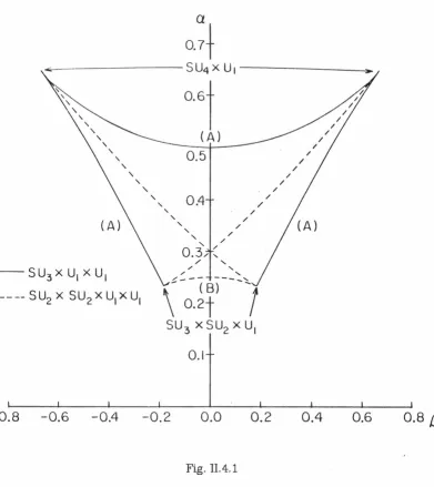
where we have listed two U1 charges in the brackets. We have underlined the singlets.The curves that represent the strata of these little groups are displayed in Fig. II.4.1.
--SU3XU1xu,
----SU2 x SU2xu1xU1
-0.8
-0.6
-0.4
0.6t
(A)0.5
0.4
'
'
'
/---
____
,
- ( 8)
-\
o.2t
I
SU3 x SU2 x U1
0.1
-0.2
0.0
0.2
Fig. 11.4.1
[image:42.613.120.511.251.690.2]A simple-minded approach to finding the boundary of the orbit space is to extremize {3 for each ex. Instead we can use the following idea. Consider a set of
</)i such that ex, {3 lies on the boundary. Make an infinitesimal variation of one of the fields C/)i. The resulting change oex/ OC/)i I 8{31 acpi forms a vector in ex, {3 space.
This vector cannot take us out of orbit space, therefore it must have vanishing component normal to the boundary. This requirement that the vector vanish or point along the orbit space boundary holds for infinitesimal variations in each 'Pi, giving us the necessary condition for a boundary point;
At a boundary point, all field components <pi must either satisfy
or must have a common value of
Partial derivatives of a and {3 with respect tori are:
4[ rP+(r 1+r2+r3+1)3]
= ---~
[r.f +r~ +r§ + 1 +(r 1+r2+r3+1)2]2
4[
ri +(r 1+r2+r3+1) ][ r ( +ri +r~ + 1+(r1+r2+rs+1)4] [rr +r~ +r~ +1+(r 1+r 2+r3+1)2]3.2.JL=
(±) 3[rl-(r 1+r2+rs+1)2]ari [rr+r~+r§+1+(r1+r2+r3+1)2]312
3[ ri +(r 1+r2+r3+1)][ r
r
+r~ +rg + 1-(r 1+r2+r3+1)3 ][rr +r~ +rg + 1+(r 1+r2+r3+1)2]512
(11.4.23)
(II.4.24)
(II.4.25)
(Il.4. 26)
To ensure that these curves really form the boundaries, we have plotted several thousand random stratum points. ·No point was found outside the boun-daries defined by the curves (A) and (B) of Fig. II.4.1.
II.4.3 LOCKI10N Qli' THE ABSOLUTE MINIMUM
Using the general formalism developed in CHII.2 we can locate the absolute minimum immediately. Since the k contours behave similarly for m2~ 0 as for
m2
>
0, we can treat all three cases together.Due to the concavity of the boundary curves of the orbit space and the con-cave shape of the k contour, the first contact can occur only at (a=13/ 20, {3=±3/ 2-v'5), the stratum of SU4xU1, or at (a=7/ 30, {3=±11 ..J30), the
stratum of SU3xSU2x U1, in agreement with the Michel-Radicati conjecture. When A1
>
0, the absolute minimum may occur at either stratum depending on the values of the other coupling coefficients. When A1<
0, the absolute minimum occurs only at the stratum of SU4x U1 . Note L11at of the two cusps with the sameex, the one with B'< 0 gets the first contact because it yields a lower value of the potential.
II.4.4 SU(N) ADJOINT REPRESENTATION
The formalism for SU5 2.1: can be extended trivially to the case of SUN adjoint representation by extending the sums to N. What is different is that there are more maximal little groups and the orbit space boundary has more cusps as the ~roup gets bigger.
The strata for the maximal little groups of SUN adjoint representation are of the form
<p
=a
(1,1, · · · ,1,;m , ;m , · · · . ;m }
where m elements have the common value a and the other (N -m) elements have the common value -am/ (N-m ). For fixed m eq. (II.4.27) represents the stratum of SUmxSUN-mx Ui. The orbit parameters for this stratum are:
m + (N-m) (N"'.::_m)4
(X =
-[m + (N-m) ( m ~2]2
N-m
m - (N -m) ( m )3 N-m {3 = ±
-[m + (N-m) ( m )2]312 N-m
The list of maximal little groups for SUN adjoint representation is:
(Il.4.28a)
(II.4.28b)
(II.4.29)
The strata for the semi-maximal little groups of SUN adjoint representation are of the form
<p = a ( r, r , · · · , r, 1.1. · · · , 1, -mr -( N -m -1) ) (II.4.30)
where m elements have the common value ar, (N-m-1) elements have the common value a, and one element is the negative sum of all the other elements. For fixed m, eq. (II.4.30) represents the stratum of SUmxSUN-m-1xU1xU1. The
orbit parameters for this stratum are:
a= mr4
+
(N-m-1)+
(mr+
(N-m-1))4 [mr2 + (N-m-1)+
(mr+
(N-m-1))2]2 '_ ± mr3
+
(N-m-1) - (mr+
(N-m-1))3 {3 - [mr2 + (N-m-1) + (mr+
(N-m-1))2]31 2(II.4.31a)
It can easily be checked that eqs. (II.4.27) and (11.4.30) satisfy the necessary
conditions for boundary points, eqs. (II.4.23) and (ll.4.24), respectively. The
cusps and curves of the boundary are shown in Fig. II.4.2 for several low N*.
Again computer generated random stratum points never appeared outside the
boundary.
It will be noted that the boundary curves corresponding to semi-maximal
little groups in Fig. II.4.2 are all concave again. One sees, using the same k
con-tour as in the previous section, that only the cusps corresponding to the
maAi-mal little groups can yield the absolute minimum, in agreement with the
Michel-Radicati conjecture. Consideration of Figs. 11.2.2 and ll.4.2 together shows
that when A1
<
0, the absolute minimum occurs only at the stratum of SUN_1x U1.When A1
>
0, the absolute minimum may occur at any of the strata of maximallittle groups, t_he choice depending on the value of the other coupling
coefficients.
Again the Michel-Radicati conjecture is found to be true for any SUN
adjoint.
(a )
( b )
~SU
5
xu1
~( c )
( d)
CHAP'l'J~H Ill TWO UliIBDUCIBIB REPRESEN'l'ATIONS
lli.1 GENERAL FORMAIJSM
When there are two irreps.
H.
and.S..
of scalar bosons~ andx
the most gen-er al re normalizable Higgs potential invariant undgen-er G x reflection can be writ-ten as+
!
[c
+ ca1(x) + c212(x) + · · ·JI
lxl 1
2+
~
[B+B1f31(~.x)+
...Jll~llllxll.
(III.1.1)While cxi and 'li specify the orbits and associated little groups of
E
and.S..
respectively, f3i specifies relative directions between orbits of
.H.
and orbits of.S..
When
x
moves on an orbit with the direction of ~ fixed, the little group of the reducible representation (H.+
.S.) changes whereas the separate little groups ofE.
and.S.
remain the same. {3i specifies the location ofx
on its orbit.Let us define
(III.1.2)
I
ho
11
~ = and I or11X11
~ =;A'> 0,
C'> 0 I (III.1.3)
B'> -
..JA'Ci
We will treat 11~
l I. I
!xi I.
~(S2J), /'i(X), and f3i(S2J,f{) as independent variables and extremize the potential with respect to these. The reasoning is similar to the one irrep case. If we choose a particular direction in ~-x space, all the orbit parameters will be determined and the potential reduces to a function of 11~11 andI lxl I:
+
!
A' I I~
11
2+
!
C'I
Ix
11
2+
~
BI 11~
I 11
Ix
I I
.
(III.1.4)The directional behavior of the potential is schematically shown in Fig. III.1.1.
The extremum for the particular choice of orbit parameters, conveniently
expressed in terms of the variables r
=
11So11*ands=11X11*. is given by the con-ditionsa
V = r (A'r2+
B's2 - M2) = 0ar
Ia
V=
s (B'r2 + C's2 - m 2)=
0as
There are four solutions;
I) r = s =O ,
II) r
=
0 , s2= m 2/ C' ,III)
IV)
(III.1.5)
(III.1.6a)
(III.1.6b)
(III. l.6c)
(III.1.6d)
To ascertain which solution is the minimum for this particular choice of direction in
So-x
space (i.e.,the directional minimum), recall that at a minimum the second derivativesa
2V = (A'r2+
B's2 - M2)+
2 A'r2ar2
Ia
2v
--=
(B'r2+
C's2 - m2)+
2 C's2as
2 •a
2v
- - = 2 B ' r s
aras
must satisfy
a2v
>
o
ar2
I(III. l. 7)
a2v
>
o
os
2 ' (III. l.Bb)(III.1.Bc)
Of course solution I is not a minimum unless M2
<
0 and m 2<
0, a case we shall not be concerned with. We see from eqs. (III.1.6) - (Ill.1.8) that solution II (pure x)is a directional minimum if
(Ill. l. 9)
Solution III (pure cp) is a directional minimum if
(III.1.10)
Solution N is a directional minimum if
(III.1.1 la)
(III.1.llb)
A'C'> (B')2 (III.1.1 lc)
for A'> 0 and C'> 0.
M2
<
0 or m2<
0 when B'< 0.From another point of view M2C' = m2B' and m2A' = M2B' represent the boundaries where the directional minimum shifts from solution N to solution II or III respectively. If solution Wis the directional minimum, extrema II and ill
are saddle points (assuming now m2
>
0, M2>
0) as indicated in Fig. III. l. lb. Inthis case evaluation of the potential at the minimum yields
(Ill.1.12)
When solution N does not satisfy the conditions (III.1.11), it occupies a saddle point and either solution II (with
Va
= -
m4/ 4C') or III (with
Va
= - M4! 4A') becomes the directional minimum.The foregoing discussion has been concerned wit~ a particular direction in
rp-x
space. As we now change the direction incp-x
space (i.e., the~ , f3i , and /'i), the location of the minimum will move around. The absolute minimum will be the lowest of these directional minima. Since
(III. l.13a)
av
=
.L
11 11
2c.
oyi
4x
'I. I (Ill. l.13b)av
18{3i
=
z-11rp1111x11
B~ I (III. l.13c)V is a monotonic function of the orbit parameters ~ , f3i , and /'i. Th~s once • The conditions (III.1.11) are only necessary conditions for solution IV to be the absolute
again the absolute minimum of V occurs at a boundary of the orbit space rather than at
a
VIaai
=
0, etc.To illustrate how determination of the absolute minimum proceeds, let's look into the simple case where
c·=
c
+
ca(x)
(III.1.14)B'= B
+
Bi{3(cp.x)Let us set
Va
(cp.x)= -
! .
(III.1.15)Then from eq. (IIl.1.12),
(III.1.16)
It can easily be shown that the above equation represents a cone in a - ?' - {3 space. That is, the potential minimizing k-surface is a cone in this problem. After some coordinate transformations, it reduces to
zz
= A1C1 (X2 _ Y2)2
Br
'
(III.1.17)where
x
= (X'+ Y')/ v'2 I(III.1.18)
C m4 Y' = ?' + C1 - kC1 I
While the coupling coefficients determine the shape and orientation of the cone, the value of k determines the location of the vertex of the cone which moves on a straight line in a - ?' - {3 space as k varies. As we decrease k from +oo, the cone begins to touch the orbit space at some k (Fig. III.1.2). This k gives the minimum energy, and the point of c_ontact gives the orbit.
y
a
Some further details concerning the cone are as follows.
i) The straight line along which the vertex of the cone moves lies on the cone
(i.e., it is a generating line of the cone.).
ii) The condition A'C' = B'2 holds on the k = 00 cone and A'C'
> B'
2 holds insideit. Recalling that A'C' > B'2 is a condition for solution N (i.e., 11So110 and
11
x
I I 0 both nonzero), we see that when this solution gives the minimumenergy, the orbit space lies entirely within the "forward" part of the cone,
i.e., the part which narrows ask decreases (Fig. III.1.2).
iii) The line along which the vertex moves is also the intersection of the two
planes
M2C'
=
m2B'and
which formed the boundary between solutions II or ID and N. These planes
slice the inside of the cone into three pieces. Only when the cone touches
the orbit space on the M2C'
>
m 2B', m2A'>
M2B' side of these planes do weget type N solutions. Such type W solutions yield the absolute minimum
energy if they occur at k
>
M4/ A'0 and k
>
m4/ C10 •While the formalism in the preceding two paragraphs is universal to all the
cases where there are three orbit parameters a, )', and (3, each different case
will have a different orbit space and different physical meaning for the boundary
surface. The formalism can be extended trivially to a general case where there
are more a's, )'1
IIl.2 'fHE GENERAL STRUCTURE OF 'I'HE ORBIT SPACE OF
nm
IRREDUCIBLEREPRESENTATIONS
While the trace of the hierarchical relationship between the levels of little groups and the concavities and dimensions of their strata observed in one irrep
case is still visible in two irrep cases, the orbit space boundary of two irreps is more complex and things are pretty much mixed. The existence of a modified resemblance can be inferred from the observation that whereas orbit parame-ters associated with each irrep tend to form warped concave boundary surfaces, orbit parameters associated with both irreps tend to destroy such behavior because with the field components of one irrep fixed (consequently orbit param-eters associated with that irrep are fixed.), one can always change the field com-ponents of the other irrep creating a volume traced by pencils. Moreover the
volume occupied by the generic stratum is not always confined by the strata of higher symmetries but the generic stratum itself surfaces on the boundaries. This "looseness" stems from the non-compactness of the representation space.
. Again an important clue leading to a description of an orbit space of two irreps is found in the Gell-Mann-Slansky conjecture [22] concerning the likely
lit-tle groups of the absolute minimum of a 4th degree Higgs potential. Since the
conjecture was made shortly before the current work started we restate it in the
following.
To state the conjecture let us define the maxi-maximal little groups:
Suppose there are two irreps H and
3...
First, we construct a list of maximal lit-tle groups and branching rules for11:
R = 1 + r1 + r2 + · · · for G'a CG
for G't> c G
For each G'i the branching rules of .S. will be
S
=
S 1+
S2+
S3+ · · ·
=
for G'a CG
for G'b c G
Then we. make a list of maximal little groups and branching rules for each si:
for G~1) C G'a
=
for
Gp
2) C G' a=
=
for G&5
>
c
G'0=
This procedure yields a list, ~G~1>, ... ;G~2>, ... :GJ4>, ... ;GJ5>, ... ; · · ·
L
ofmaxi-maximal little groups. Repeating the same procedure staring from
S..,
we obtain another list of maxi-maximal little groups, which is different from the
previous list.
The Gell-Mann-Slansky conjecture states that the minimum of a fourth
maxi-maximal little groups, which is made of the union of the two lists.
In the previous chapter we have seen that the potential minimizing k-surface for a Higgs potential of tw_o irreps which has separate reflection sym-metries in addition to the symmetry of the gauge group is a hyper-cone. This
implies that if the Gell-Mann-Slansky conjecture is to hold for such a class of Higgs potentials then the strata of maxi-maximal little groups must occupy most protrudent portions, i.e., cusps, convex curves and surfaces etc., of the orbit space boundary. Specific examples will be given in the following chapters.
To help the reader to understand the abstract statements made above, let us briefly explain dimensionalities of strata of two irreps. Suppose the branch-ing rules for two irreps,
E
and S, under G'cG areIf
E.
contains one singlet and.S.
one singlet of G', then the stratum will be a point in the orbit space. IfE.
contains one singlet and.S.
two singlets of G' or vice versa, the stratum will normally be a curve in the orbit space, though there areexceptions. If
E.
contains one singlet and.S.
three singlets of G' or vice versa, the stratum is likely to be a two-dimensional surface. IfE
contains two-singlets and.S..
two singlets of G', the stratum is likely to occupy a three-dimensional volume.ill.3 APPIJCATION TO SU(N) ADJOINT +VECTOR REPRESENTATIONS
1'}.3.1 IIlGGS POTENTIAL FOR SU(5) 24
+
~In this chapter we apply the general formalism derived in the previous
chapter
lo
the
case of
SU0adjoint
+
vectorrepresentations.
This particularproblem has been solved by many people [32] ever since Georgi and Glashow [6] formulated the grand unification theory based on SU5 symmetry. In other
branches of physics [9], namely in the second order phase transition occurring in order-disorder phenomenon [10], the spontaneous symmetry breaking
prob-lem already became so complicated that more powerful means were required. But in elementary particle physics it was the appearance of grand unification theories that prompted the need of more powerful methods than conventional ones. There was just no hope of minimizing the scalar potential with conven-tional methods when the representation of the scalar bosons is as huge as the ones introduced in 8010 or E6 unification theories [33].
We will consider two scalar fields: (/)ii, which transforms as the
24-dimensional adjoint representation, and Xi, which transforms as the 5-dimensional (complex) vector representation. The most general renormalizable Higgs potential invariant under SUr-, x reflection is
where we have represented the
.21:
as a 5 x 5 traceless hermitian matrix. Because