Developing Evaluation Module for Battery Lifetime

2016 International Conference on Artificial Intelligence: Techniques and Applications (AITA 2016) ISBN: 978-1-60595-389-2

Developing Evaluation Module for Battery Lifetime

Jing ZHANG

, Kenji TANAKA

and Shen-ming GU

*

Key Laboratory of Oceanographic Big Data Mining & Application of Zhejiang Province, Zhejiang Ocean University, No.1, Haida South Road, Lincheng, Changzhi Island, Zhoushan, Zhejiang,

316022, P.R. China

2

Department of System Innovation, Graduate School of Engineering, The University of Tokyo, 7-3-1 Hongo, Bunkyo-ku, Tokyo 113-8656, Japan

*Corresponding author

Keywords: Battery performance, Evaluation, Model, Simulation.

Abstract. Lithium-ion batteries (LiBs) have seen increasing use in automobiles and buildings over the past decade. Usable lifetimes of several years are sufficient for LiBs used in electronic devices, but infrastructure applications require lifetimes measured in decades. Users of LiBs are faced with uncertainty about LiB lifetimes, which hinders the spread of LiBs. Predicting LiB performance degradation and evaluating useful lifetimes by examining present performance is therefore important for planning. Our research group has developed an evaluation model for LiBs that comprises an empirically obtained degradation speed database and a method for recognizing LiB usage patterns.

Introduction

The performance of lithium-ion batteries (LiBs) has drastically improved over the past decade, and the cost of LiBs has also decreased. This has made LiBs practical for both consumer applications and for use in various electrical infrastructure systems, such as electric vehicles (EVs) [1]. Transportation applications are still in early stages being adopted, with LiBs of around 20 kWh being equipped in EVs and 2–5 kWh batteries being used for plug-in hybrid electric vehicles (PHEVs). Stationary applications, such as secondary use of EV LiBs for home energy management and for building and renewable energy generators, are also drawing increasing attention. Even though infrastructure applications demand 10–15 year battery lifetimes, methods for ensuring long-term LiB performance have yet to be established. This increases uncertainty about LiB lifetimes and is one of the factors preventing wider adoption of LiBs for infrastructure use. The spread of LiB-based energy management systems requires establishing methodologies that ensure LiB value by evaluating long-term performance.

Literature Review

Developing an evaluation model for LiB lifetime requires defining key performance indicators for LiB performance. The degradation mechanism of individual LiB materials has previously been studied [2, 3] as has the relationship between the main factors of degradation and the discharge curve line [4–9]. Other studies have developed models for LiB lifetime estimation under constant environmental conditions [10]. Recent studies have examined LiBs degradation when the batteries are used for leveling the output power of renewable energy generators [11].

Definition of LiB Performance

We use energy density E [J] and power density P [W] as key performance indicators for LiBs. E influences available energy, and P influences output power, such as the driving power of an EV. Using Eq. (1), E can be derived from the electric capacity Q [Ah]. In Eq. (2), V and Vaverage are voltages, and I is the current. P can be derived from the internal resistance R [ohm] in Eq. (1). The present value for an LiB can thus be evaluated from Q and R.

( ) average

E





0

( )

P  V I V   R I I (2)

Performance Evaluation

Evaluating LiB performance requires focusing on two aspects of Q and R, namely, present and future performance. Evaluating present performance detects abnormal degradation, such as that due to an internal short circuit. If abnormal degradation is detected, the LiB should no longer be used. Such evaluations conventionally require measuring electrolyte decomposition in the LiB, making them unsuited to practical applications in which continual use is desired.

Evaluating future performance predicts how long the LiB will last under certain conditions, and the results influence the evaluation of an LiB’s value. Forecasting LiB lifetime requires simulating LiB degradation, expressing degradation of Q and R as functions of time.

Evaluation of Present Performance

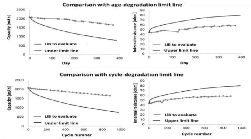
Evaluations of present performance determine whether the decreases in capacity Q and the increases in internal resistance R are within the range of normal degradation caused by use. Figure 1 shows an example evaluation of present performance. Q and R are compared with baseline values in two degradation situations: degradation due to age, which is shown in the upper part of, Figure 1 and degradation due to charge/discharge cycling, which is shown in the lower part of the figure. Evaluation of Q is shown at the left. Values of Q below the “lower limit line” indicate abnormal degradation of capacity. R is shown at the right. Values of R above the “upper limit line” indicate an abnormal increase in internal resistance.

Degradation Model Development

This section develops an interim degradation model for Q and R and uses the model to analyze data from a degradation experiment on an LiB (18650 type). Eqs. (3)–(5) give a degradation model for capacity ΔQ, which is expressed as the sum of ΔQcycleand ΔQtime. ΔQcycleis the decrease in capacity

due to charge/discharge cycles and is the product of the cycle number cyclenQc and the degradation speed fQc, whose independent variables are state of charge SOC, temperature T [°C],charge/discharge

rate C, and, possibly, other factors. ΔQtime is the decrease in capacity due to elapsed time from the start

of use. It is expressed as the product of elapsed time and the degradation speed fQt, whose independent

variables are the same as those of fQc. Similarly, the increase in internal resistance ΔR (Eqs. (6)–(8)) is

expressed as the sum of ΔRcycle, the degradation of R caused by charge/discharge cycles, and ΔRtime,

the degradation of R caused by elapsed time from the start of use.

cycle time

Q Q Q

     (3)

( , , ) nQc

cycle Qc

Q f SOC T C cycle

   (4)

( , , ) nQt

time Qt

Q f SOC T C time

   (5)

cycle time

R R R

     (6)

( , , ) nRc

cycle Rc

R f SOC T C cycle

   (7)

( , , ) nRt

time Rt

R f SOC T C time

   (8)

Degradation Experiment on 18650-type LiB Cells

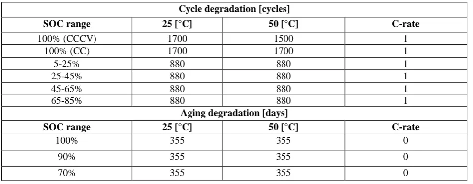
This and the following two sections discuss development of a degradation speed database. Developing the database required experimentally measuring degradation of a 18650-type LiB. Table 1 shows the degradation conditions of the LiB cells used in the experiment in terms of number of cycles and elapsed usage time. Here, cycle time is derived by dividing the accumulated discharge magnitude by the capacity of the LiB cell. Two types of degradation were used in the cycle degradation experiment, namely, degradation with 100% and 20% ranges of change in SOC. Furthermore, two charge/discharge conditions of the LiB cells with 100% SOC range were set: constant current–constant voltage (CCCV) and constant current (CC). Four phases of SOC range were set for LiB cells with a 20% range of change in SOC. Age-degraded LiB cells were experimented on with SOC at 70%, 90%, and 100%. Temperatures were 25 and 50 °C.

Table 1. Degradation conditions of cycle-degraded LiB cells.

Cycle degradation [cycles]

SOC range 25 [°C] 50 [°C] C-rate

100% (CCCV) 1700 1500 1

100% (CC) 1700 1700 1

5-25% 880 880 1

25-45% 880 880 1

45-65% 880 880 1

65-85% 880 880 1

Aging degradation [days]

SOC range 25 [°C] 50 [°C] C-rate

100% 355 355 0

90% 355 355 0

Development of the Capacity Degradation Speed Database

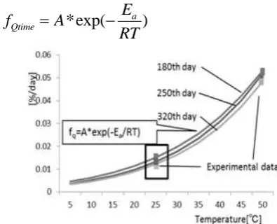
This section discusses development of the capacity degradation speed database. Using cycle degradation data at 25 and 50 °C and Arrhenius’s formula (Eq. (9)) gives the lithium-ion activation energy, from which one can derive the degradation speed between 25 and 50 °C. Figure 2 shows the speed of capacity degradation for an LiB with 70% SOC after 180, 250, and 320 days. Figure 2 indicates that higher temperature increases the degradation speed and that degradation slows over time. Table 2 shows degradation speeds at 70%, 90%, and 100% SOC and indicates that degradation speed increases with SOC range.

*exp( a ) Qtime

E

f A

RT

  (9)

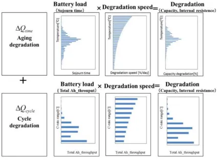
Figure 2. Capacity degradation speed at different. Figure 3. Concept of deriving capacity degradation.

Table 2.Capacity degradation speed [%/day] (0C, 0–320th day).

SOC 25 [°C] 50 [°C]

100% 1.54E-2 -

90% 1.50E-2 5.13E-2

70% 1.21E-2 4.84E-2

Table 3. Capacity degradation speed (1C, 25 °C, 0–320th day).

SOC Cycle degradation speed [%/cycle]

5-25% 6.27E-3

25-45% 4.45E-2

45-65% 3.74E-3

65-85% 9.06E-3

0-100% 2.38E-2

Figure 3 shows the calculation of cycle degradation speed. Because aging degradation accompanies cycle degradation in the LiB cell data, ΔQtime is subtracted from the ΔQ of cycle-degraded LiB cells to obtain ΔQcycle. Cycle degradation speed is derived by dividing ΔQcycle by the accumulated number of cycles. Table 3 shows the cycle degradation speed on the 320th day at 25 °C as an example. In general, cycle degradation speed increases as the range of SOC widens.

Development of Internal Resistance Speed Database

We developed a similar database of degradation speeds for internal resistance fRc related to cycle

degradation and fRt related to aging degradation. Table 4 shows the degradation speed fRt at each range

of change in SOC at 25 °C. Degradation speed fRt increases with SOC range, which indicates a

positive correlation between SOC range and degradation speed of internal resistance.

Figure 4. Concept of deriving capacity degradation.

Table 4. Internal resistance degradation speed at 25 °C.

SOC range Cycle degradation speed at 25 °C

5-25% 1.66E-2

25-45% 2.47E-2

45-65% 1.83E-2

65-855 2.92E-2

Setup of Stationary Usage Patterns

Table 5. Usage conditions of the stationary battery.

Average SOC [%] 49

Charge/discharge ratio to its capacity [%] 64

Average C-rate [C] 0.07

Maximum C-rate [C] 0.67

Average temperature [°C] 17

Maximum temperature [°C] 27

Figure 5. Discharge time at each C-rate range over 1 year. Figure 6. Dwell time at each SOC range over 1 year.

Conclusion

We developed an evaluation model for predicting LiB lifetime. The model includes the following: a degradation model for capacity Q and internal resistance R,

an empirically obtained degradation speed database, and LiB usage patterns, based on use-history analysis.

References

[1] T. Takuya et al. ‘Route Search and Evolution Method Including Charging Plan for Electric Vehicles’ International Journal of Automation technology Vol.8 No.5 698-704 (2014).

[2] J. Abe, H. Haruna, E. Seki, K. Nishimura, K. Kohno, T. Hirasawa, S. Itoh, T. Horiba, and T. Yoshiura, The 52nd Battery Symposium in Japan, 67(3A22), October17-20, Tokyo. (2011).

[3] S. Lee, J. Kim ‘State-of-charge and capacity estimation of lithium-ion battery using a new open-circuit voltage versus state-of-charge.’ J. Power Sources 185, 1367-1373 (2008).

[4] Johnson, V.H. Battery performance models in ADVISOR. J. Power Sources 110, 321-329 (2002).

[5] Shen, W.X.; Chan, C.C.; Lo, E.W.C.; Chau, K.T. ‘A new battery available capacity indicator for electric vehicles using neural network. Energy Convers.’ Manage. 43, 817-826 (2002).

[6] Discharge behavior. In Proceedings of 7th International Conference on Artificial Neural Networks, Lausanne, Switzerland 1095-1100 (1997).

[7] I. Snihir et al. ‘Belfadhel-Ayeb and P. H. L. Notten, Battery open-circuit voltage estimation by a method of statistical analysis. J. Power Sources, vol. 159, no. 2, 1484-1487 (2006).

[9] M. Abe et al. ‘Lifetime prediction of lithium-ion batteries for high-reliability system.’ Hitachi Rev 94:334-337 (2012).

[10] F. Gao Et Al Kinetic behavior of LiFePO4/C cathode material for lithium-ion batteries.’ Electrochim Acta 53:5071-5075 (2008).