2017 International Conference on Computer Science and Application Engineering (CSAE 2017) ISBN: 978-1-60595-505-6
Volume Rendering of Planet-scaled 3D Atmospheric
Data on Virtual Globes
Lianqing Yu*
National Meteorological Center, China Meteorological Administration, 100081 Beijing, China
ABSTRACT
Although texture slicing based volume rendering method has been widely used in data visualization, applying it to render atmospheric data that span entire globe has always been a challenging task. The difficulties are threefold. First, conventional volume rendering methods are used to process data referenced in a Cartesian coordinate system, whereas atmospheric data are georeferenced to a geodetic coordinate system. This difference brings about complications in texture sampling. Second, planet-scaled atmospheric data, especially those in high resolution, exacerbate performance issue in rendering time complexity. Third, spherical shaped bounding volume of Earth’s atmosphere makes the calculation of proxy geometry difficult. In this paper, a new method is proposed to tackle the challenges aforementioned. The coordinates of volume vertices and textures are represented in spherical coordinate system to avoid the accuracy loss due to conversion between Cartesian and geodetic coordinate system. The calculation of proxy geometry is worked out. The proposed method is tested by being implemented into a rendering engine visualizing atmospheric data set.
INTRODUCTION
In the field of atmospheric science and geosciences, volume rendering [1] is a popular method for data presentation and analysis. The method has been incorporated into scientific research tools like IDV [2], VAPOR [3], Met.3D [4], and ParaView [5]. These tools are designed to render regional uniform grids except for ParaView, which supports spherical grid data. Conventional volume rendering methods [6] [7] [8] deal primarily with structured grids. With the popularity of digital Earth applications, research emphasis has been extended to the methods for unstructured grids [9]. Liang et al. proposed the concept of spherical rendering texture [10] to render atmospheric data like clouds on a virtual globe platform. Their work differs from the work herein in two ways. First, their rendering results (Figure 11 of [10]) show that the geographic range of the data set is less than half hemisphere, whereas the range our work deals with is global. Second, they use a ray-casting method, contrary to the slicing method used in this work. Xie et al. proposed a ray-casting method that traverses geodetic grids using 2D connectivity information [11]. They later applied the method to render large scale climate simulation data using distributed supercomputing system [12]. Their work differs from ours in that we use curvilinear grids instead of geodetic grids, and we select slicing instead of ray-casting method.
these methods,texture-based slicing is a viable technique in that three-dimensional (3D) texture sampling supported by modern graphic processing units (GPUs) makes it convenient to use a set of parallel polygons [9] [17].
The work proposed in this paper focuses on applying texture-based slicing method to render planet-scaled atmospheric data. In order to achieve good quality and performance, a couple of efforts have been made to address the difficulties in the rendering process. The work herein has accomplished the followings: First, vertex position coordinate and texture coordinate are represented in spherical coordinate system to avoid the loss of accuracy resulted from conversion between Cartesian and geodetic coordinate system. Second, the calculation of proxy geometry as the intersection between the view aligned slice plane and the bounding volume of the data is worked out. Third, the proposed method is integrated into a cross-platform rendering engine that is capable of rendering real-world atmospheric data.
VOLUME RENDERING FOR SPHERICAL SHAPED DATA
Coordinate Transform between Geodetic and Cartesian Coordinate System
A typical GIS system usually makes use of geodetic coordinate system that is described in terms of longitude (λ), latitude (δ) and altitude (ρ). Analogously, numerical weather prediction models employ a coordinate system similar to geodetic coordinate system in that pressure or terrain following sigma-pressure is used as vertical axis unit instead of altitude [18]. Sigma is an independent variable in the model that denotes pressure at an altitude scaled with surface pressure. A hybrid sigma-pressure coordinate allows for continuous fields to be represented at lowest layer. In graphics hardware pipeline however, a position is commonly represented by a triple set (x,y,z) in Cartesian coordinate system. Fortunately, spherical coordinate system can be used to serve as a bridge between geodetic and Cartesian coordinate system. Equation (1) describes the relation between the two systems.
2 2 2 z y x e , z x tan , 2 2 2 sin z y x y (1)
wheree is Earth radius.
Spherical Texture Coordinate System
Similar to position coordinate, texture coordinate should also be adapted to geodetic coordinate system. In traditional volume rendering where the bounding box takes the form of a cuboid, texture coordinate of a vertex can be obtained by normalizing its position coordinate. For rendering of a data set whose bounding volume takes the form of a spherical shell, the method does not work anymore because the cubic texture space does not correspond to the spherical position space.
To deal with this issue, a new method is proposed to obtain the texture coordinate of a vertex by normalizing its geodetic coordinate as described in Equation (2)
min max min x t , min max min y t ,
max minmin
s
where
tx,ty,tz
is the vertex’s texture coordinate, and
min,max
(
min,max
,
min,max
respectively) represents range of longitude (latitude, altitude respectively). The variable s is the stretch factor in vertical direction and introduced to exaggerate the altitude range. In this way, texture coordinate system can be connected to geodetic coordinate system.The linear interpolation of texture coordinate in geodetic space does not suffer from the pole-problem inherent in curvilinear grids. The reason is that the topology of sliced polygons near pole area is independent of resolution of texture coordinate. Indeed the density of vertices of sliced polygons near pole area is low. An alternative approach to texture interpolation is to use map projection. However a problem with this method is the time complexity as map projection is computationally more expensive than linear interpolation and may result in a bottleneck in proxy geometry calculation. In addition, using map projection does not increase calculation accuracy of texture coordinate as all the calculations are performed in 3D.
Spherical Shell
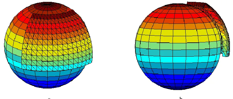
For texture-based slicing methods, a bounding box that fully contains the data volume has to be determined in the first place. For atmospheric data surrounding the Earth, the bounding volume takes on the shape of a thin spherical shell, which is composed of two spherical surfaces (inner and outer surface) and four walls on the edges. Taking into account of the fact that the upper limit of tropopause is about 18 kilometers (km) and Earth radius is about 6381 km, the thickness of spherical shell is very small.
[image:3.612.116.492.401.561.2]a b
Figure 1. The front view (a) and side view (b) of a spherical shell.
Figure 1 gives an illustration of a spherical shell in front view (a) and side view (b). The vertical stretch factor is set as 35 for better visualization. The introduction of the spherical shell lays a mathematical foundation for the calculation of proxy geometry.
Calculation of Proxy Geometry
two layers (Figure 1). The intersection vertices are obtained through a line-plane intersection test between all the edges of the mesh and the slice plane.
There are three major cases as for the intersections:
1. The slice plane intersects with inner surface of the shell only, the intersection is a couple of polygonal pieces.
2. The slice plane intersects with outer surface of the shell only, the intersection is a disk.
3. The slice plane intersects with both outer and inner surface of the shell, the intersection is either
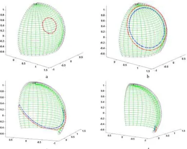
a) An annulus (happens in the near part of the shell away from the eye). b) An arched band (happens in the middle part of the shell).
c) A couple of polygonal pieces (happens in the further and outer part of the shell). Figure 2 illustrates all the cases. Figure 2a (2b, 2c, 2d respectively) corresponds to case 2 (3a, 3b, 3c respectively). The spherical shell is drawn as a mesh in gray for outer surface and in green for inner surface. The vertices of the intersection of the plane with outer surface are drawn in red, and those with inner surface are drawn in blue.
a b
[image:4.612.97.481.287.593.2]c d
Figure 2. The illustrations of all the cases of intersections between view-aligned slice plane and spherical shell.
Performance Considerations
rendering performance. For atmospheric volume data in planet scale, an upper limit of 32 edges along the longitude or latitude direction suffices to keep the shape of the spherical shell. The simplification of the spherical shell also makes the performance of our algorithm independent of the resolution of the data, which may contain thousands of grids along longitude or latitude direction in the case of a high-resolution grid field. A proxy geometry can also be simplified by reducing the number of its vertices in order to increase rendering speed. For example, the number of vertices in Figure 2b can be decremented to 16 per circle without changing its annulus-like shape.
IMPLEMENTATION AND RESULTS
In the implementation of the proposed method, scalar grid data are stored in a 3D array used as volume texture data. If grid data dimension exceeds the maximum texture size supported by the hardware driver, the whole grid is divided into multiple bricks. For each brick, data extension in geodetic coordinate system and dimensions in all three axes are calculated so that data value of a given grid point can be interpolated. After this preparation, sample count is determined by computing the nearest and furthest distance between the spherical shell and the eye as well as corresponding grid points count within this range. Next, the whole volume is sliced into multiple images defined by the intersection polygons. This slicing operation is done in a back-to-front order. Volume texture type is 8 bits per voxel. Transfer function is implemented as a color lookup table (CLUT), which is created as a 1-D texture and passed to GLSL (HLSL respectively) shader as uniform (constant buffer respectively) variable.
a b
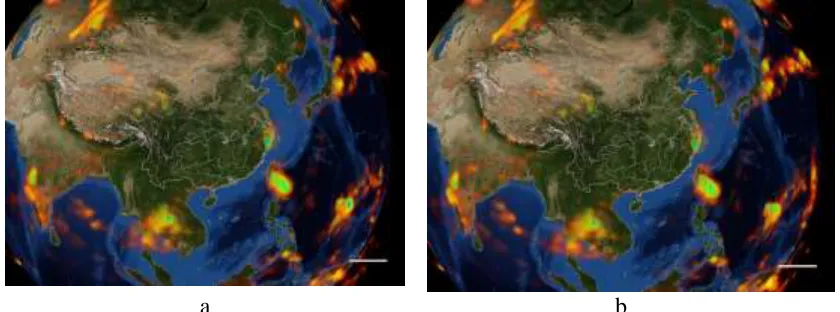
Figure 3. Rendering quality comparison of our method implemented with (a) and without (b) vertex reduction of intersection polygons. The data set is cloud water mixing ratio on 12:00 UTC September 13,
[image:5.612.92.512.399.555.2]2016, when typhoon Maranti was at its peak intensity.
values and green color large values. With this configuration, typhoon Maranti can be easily identified on the south-east of Taiwan. Figure 3 also provides a comparison of rendition quality of the method with (a) and without (b) performance optimization by reducing vertices of intersection polygons. As we are cautious not to change the shape of the intersection polygons during vertex reduction, the rendering results are comparable.
Performance Analysis
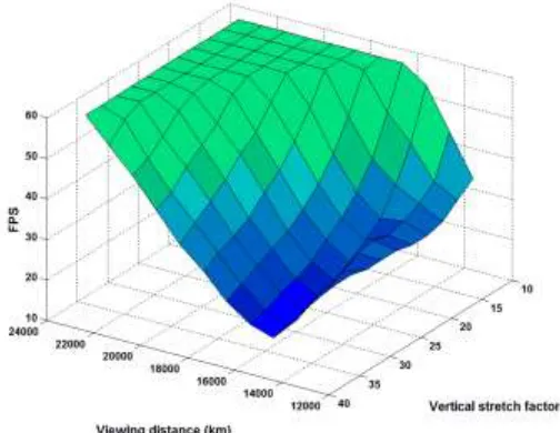
[image:6.612.176.428.248.443.2]Performance testing is necessary to evaluate the efficiency of the proposed method. In the experiments, frame per second (FPS) is used as the benchmark. It is found that the rendering performance depends on viewing distance between the camera and the volume, as well as the vertical stretch factor [17].
Figure 4. The rendering performance measured by frame per second (FPS) against viewing distance and vertical stretch factor.
The experiment results shown in Figure 4 verify the conclusion that rendering performance is affected by the two factors mentioned in the beginning of this section. First, the frame rate drops monotonously as the viewing distance decreases. It drops earlier for large vertical stretch factors than for small factors. Second, performance decreases as vertical stretch factor increases for viewing distance smaller than a certain threshold, in this case 24000 km. In all, rendering performance is adversely affected by small viewing distance and large vertical stretch factor. Meticulous readers may find that the minimum frame rate does not correspond to smallest viewing distance. The reason is that for viewing distance that is smaller than a threshold, 6000 km in our scene setup, only a small proportion of the volume is visible on the screen.
a b
Figure 5. Performance comparison between our method and the ray-casting method proposed in [10].
Figure 5 provides a performance comparison between our method (labeled as slicing) and the ray-casting method proposed in [10] (labeled as ray-casting) using Katrina data set (a) and Maranti data set (b). The experiment setup is identical to that of Figure 4 with the exception that the vertical stretch factor is fixed at 20. Sampling rate is identical for both methods. The ray-casting method is a faithful implementation of [10] and no optimization techniques such as pre-integration, empty-space leaping are included. For Katrina data set, the geographic area is 96.13W~83.09W west-east, 22.77N~34N south-north and the dimension is 315x309x34. For this data set, the performance of the two methods is comparable. For Maranti data set introduced in the previous section, our slicing method outperforms the ray-casting method. A reason for the result is that a significantly larger number of fragments need to be processed for global data set, and fragment shader of ray-casting method is computationally more expensive than that of slicing method.
CONCLUSIONS
[image:7.612.102.494.205.347.2]tested by being integrated into a cross-platform graphics rendering engine and doing volume rendering of real-world data set.
In the future, we would like to improve the method by implementing the computationally intensive work such as the intersection between the slice plane and the shell in GPU.In detail, the slice plane is used as the proxy geometry and passed to the fragment shader, where the intersection is obtained as two ellipses in either normal (Figure 2b) or degenerate form (Figure 2a, 2c, and 2d). If a fragment projects into the band defined by the two ellipses, its color is calculated. Otherwise, it is discarded. This method not only takes advantage of parallel processing capability of modern graphics hardware, but also decouples grid size and proxy geometry complexity.
REFERENCES
1. K. Engel, M. Hadwiger, J. Kniss, C. Rezk-Salama and D. Weiskopf. 2006. Real-Time Volume Graphics, first ed., A K Peters.
2. D. Murray, J. McWhirter and Y. Ho. 2009. "The IDV At 5: New Features and Future Plans," in
Proceedings of 25th Conference on International Interactive Information and Processing Systems (IIPS) for Meteorology, Oceanography, and Hydrology, pp. 7B.5.
3. J. Clyne, P. Mininni, A. Norton and M. Rast. 2007. "Interactive Desktop Analysis of High Resolution Simulations: Application to Turbulent Plume Dynamics and Current Sheet Formation," New Journal of Physics, 9(8):301-329.
4. M. Rautenhaus, M. Kern, A. Schafler and R. Westermann. 2015. "Three-Dimensional Visualization of Ensemble Weather Forecasts - Part 1: The visualization tool Met.3D," Geoscientific Model Development, 8(7):2329-2353.
5. U. Ayachit. 2015. The ParaView Guide: A Parallel Visualization Application, Kitware.
6. B. Cabral, N. Cam and J. Foran. 1994. "Accelerated Volume Rendering and Tomographic Reconstruction Using Texture Mapping Hardware," in Proceedings of the 1994 symposium on volume visualization, pp. 91-98.
7. J. Kruger and R. Westermann. 2003. "Acceleration Techniques for GPU-based Volume Rendering," In Proceedings of the 14th IEEE Visualization, pp. 287-292.
8. S. Roettger, S. Guthe, D. Weiskopf, T. Ertl and W. Strasser. 2003. "Smart Hardware-Accelerated Volume Rendering," In Proceedings of the Eurographics/IEEE TVCG Symposium on Visualization, pp. 231-238.
9. C. Silva, J. Comba, S. Callahan and F. Bernardon. 2005. "A Survey of GPU-Based Volume Rendering of Unstructured Grids," Brazilian Journal of Theoretic and Applied Computing, 12(2):9-29.
10. J. Liang, J. Gong, W. Li and A. N. Ibrahim. 2014. "Visualizing 3D Atmospheric Data with Spherical Volume Texture on Virtual Globes," Computers & Geosciences, 68:81-91.
11. J. Xie, H. Yu and K.-L. Mu. 2013. "Interactive Ray Casting of Geodesic Grids," Eurographics Conference on Visualization (EuroVis), 32(3):481-490.
12. J. Xie, H. Yu and K.-L. Ma. 2014. "Visualizing Large 3D Geodesic Grid Data with Massively Distributed GPUs," IEEE Symposium on Large Data Analysis and Visualization, Paris 2014, pp. 3-10.
13. P. Lacroute and M. Levoy. 1994. "Fast Volume Rendering Using a Shear-Warp Factorization of the Viewing Transform," In Proceedings of SIGGRAPH '94, pp. 451-458.
14. L. A. Westover. 1991. "SPLATTING: A Parallel, Feed-Forward Volume Rendering Algorithm," Chapel Hill.
15. N. Max, P. Williams, C. Silva and R. Cook. 2003. "Volume Rendering for Curvilinear and Unstructured Grids," in Proceedings of Computer Graphics International 2003, pp. 210-215. 16. J. Kruger. 2010. "A New Sampling Scheme for Slice Based Volume Rendering," in Proceedings of
the 8th IEEE/EG international conference on volume graphics, pp. 1-4.
17. R. Fernando. 2004. GPU Gems: Programming Techniques, Tips and Tricks for Real-Time Graphics, first ed., Addison-Wesley Professional.
![Figure 5 provides a performance comparison between our method (labeled as slicing) and the ray-casting method proposed in [10] (labeled as ray-casting) using](https://thumb-us.123doks.com/thumbv2/123dok_us/287846.1029581/7.612.102.494.205.347/figure-provides-performance-comparison-labeled-slicing-casting-proposed.webp)