Origin Destination Trips for Human Mobility Based on Twitter

2017 2nd International Conference on Computational Modeling, Simulation and Applied Mathematics (CMSAM 2017) ISBN: 978-1-60595-499-8

Origin-Destination Trips for Human Mobility Based on Twitter

Xiao-ya SHAN

and Jing-jing SONG

Systems Science Institute Beijing Jiaotong University, Beijing 100044, China

*Corresponding author

Keywords: Human mobility, Twitter, Data mining, Trip distribution.

Abstract. The availability of massive anonymized datasets provides a novel insight for understanding human mobility which is important to disease prevention, city planning and traffic forecasting. Most relevant studies employ call detail record (CDR) data with convenient collection but low location resolution. Twitter data, as an alternative, can be located within ten meters. This paper focuses on studying the human mobility with Twitter data in Milano, Roma and Venezia. Firstly, the stay points of Twitter users are extracted and classified into three types: Home, Work and Other. Then, Grid-based cluster algorithm is proposed to clustering these stay points into different stay regions. Next, the trips of Twitter users are divided into three categories: Home-Based Work (HBW), Home-Based Other (HBO) and Non-Home Based (NHB). Finally, the Twitter users’ trips are plotted and visualized by Geographic Information System (GIS). Computational results explicit that the tendency of trips length and times are in accordance with Zipf’s law.

Introduction

Our ability to correctly analyze the urban daily trip demand, recognize the trajectories and patterns humans follow during their daily activities, is not only a grave challenge, but also of importance for public health, city planning [1,2], emergency prevention [3], economic development estimating [4] and traffic demand management during big events [5]. Consequently, enhancing this ability is conducive to promote the construction of smart city.

The highly penetration of smartphones, along with rapid development in location technology put forward higher requirements to understanding human mobility. Most papers made some efforts in this area based on the CDR data [6-11], Wi-Fi data [12], RFID data [13,14] and GPS data [15,16]. Although studies based on these data have carried out in-depth research on human mobility dynamics, these data involves privacy concerns and data access restrictions [17].

Recently, various mobile applications provide location function, allowing people to share their locations on the internet, such as the online social networking and micro blogging applications twitter, which provide an ideal data source for human mobility research. Additionally, tweets with geotag has high location resolution lower than 10 meters, which are more accurate than CDR data. There have been several research demonstrating that Twitter data can be a reliable source for human mobility patterns from different perspectives. At individual level, the displacement distribution, the radius of gyration, and the Zipf’s law of visitation frequency of human spatial mobility were analyzed [18]. A few studies concentrated on spatial distribution of tweets and densities within cities at city level [19].

In this paper, we analyze a large twitter data set of several cities in Italy. Then, we present an overview of the methods to recognize the stay region of user and extract the daily trips. Next, the empirical results and relative analyses is displayed. Lastly, conclusions are given together with recommendations for future research.

Data and Methods

Twitter Data

Big Data Challenge. The format of data is JSON, each record contains the tweets language, created time, geometry type, coordinate, timestamp, modified, entities, anonymous user ID. The coordinates of the records are GPS location, with an accuracy less than 10m, which are more precise than CDR data with accuracy about 200-300m.

Extracting Stays

The first step in the data processing pipeline is to filter the raw data. We only analyze the users with more than 50 tweets during the observation. Furthermore, we wish to identify the users’ stays locations and pass-by locations. A stay location is a geographical region where a user stayed over a time threshold with a spatial threshold. The time threshold is the minimum stay time in a stay location. The spatial threshold is a roaming distance of a stay location as 300m. The position of the stay location is defined as the centroid of all the records belongs to this stay location [10].

The second step is to cluster the stay locations into stay regions because of some stay locations refer to a same interested region in practice. We use the grid-based cluster algorithm to cluster the stay locations into stay regions [20]. The procedure is as follows: First, we segment the entire region into square grids with width of d/3, d is the stay region size as 300m. Second, project all the stay locations into each grid. Third, iteratively cluster the unassigned grid with maximum stay locations and its’ all unassigned neighbor grids to a new stay region. Finally, calculate the centroid of all the stay locations in the same stay region as the coordinate of this stay region. What’s more, we filter the users have one stay region at least.

Identifying Location Type: Home, Work, Other

To analyze the human mobility, it’s necessary to identify the type of each location user visited. For each stay region, we categorize it as Home, Work, or Other [9]. We recognize the most frequently visited stay location during weekday nights (between 8pm of first day and 9am of second day) and weekend as Home.

For no home stay location, we define it as potential work stay location if its start time is during the weekday 9am to 8pm. Based on the historical evidence, trips with longer distance are more likely to be work trips than those with shorter distance for the same visitation frequency. So we label a potential work stay location as Work, if the distance between this location and home location larger than 500m. Besides, more than 3 times visitation during the observation period for a work location is required. Otherwise, the stay location is labeled as Other. If the users have few records, we can’t analyze his mobility, so we filter the users have at least 10 home visitations during the observation period.

Extracting Trips and Identifying Trip Type

After characterizing the stay location of users, we can extract the trips of users according to the time series. For different travel purposes, we categorize the trips into three types: HBW, HBO and NHB [9]. HBW trip represents the trip from Home location to Work location or from the Work location to Home location. HBO trip is the trip between Home location and Other location. NHB trip is the trip without the Home location.

For each user, we set the trip occurring period as a 24 h period beginning and ending at 3 am, a trip is made once there are two consecutive different stays occurring within this period. We define the create time of the origin record as 𝑡𝑖, the create time of destination record as 𝑡𝑖+1, then the trip departure hour equals to the median of the time window [𝑡𝑖, 𝑡𝑖+1]. Most notably, we presume that a daily trip starts and ends each 24 h period at home location, so if the first (last) trips in each day not start (end) at home, we set it at home, and the departure time of trip is set as the median of the time window [3am, 𝑡_𝑖+1] ([𝑡_𝑖, 3am]).

Results

users. Based on the distribution, we can study the trip demand for future urban planning. As shown in Figure 1, we observe a Zipf’s law of the trip frequency, i.e. 𝑃(𝑇) can be described by a power-law function 𝑃(𝑇)~𝑇−𝛼. Also it’s obvious that the distribution features are familiar for different cities.

We then explore the users’ trip length in different cities. Also the trip length follow Zipf’s law which shown in Figure 2. The average trip length by purpose and cities is displayed in Table 1. The similar results for three cities illustrate that we can use Twitter data to compute the average travel distance because there are no actual average travel length data in Italy.

(a) Milano (b) Roma (c) Venezia

Figure 1. Distribution of trip times for users in different Italian cities.

(a) Milano (b) Roma (c) Venezia

Figure 2. Distribution of trip length for users in different Italian cities.

Table 1. Average trip length by purpose for Milano, Roma and Venezia. The unit of trip length is kilometers.

City HBW HBO NHB ALL

Milano 5.96 4.23 4.49 4.42

Roma 5.26 4.59 5.03 4.81

Venezia 7.07 5.11 5.08 5.17

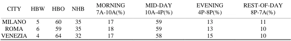
As mentioned in Section Extracting Trips and Identifying Trip Type, we label the trip into three types, HBW, HBO and NHB. Figure 3 illustrates the distribution of hourly departure time distribution for HBW, HBO, NHB and total average trips for Milano, Roma and Venezia. The laws of the three cities are consistent for different trip purposes. Furthermore, Figure 3 displays the morning peaks of HBW trips, which consistent with the practical rule. Table 2 shows a comparison of average trips by purpose and period of the day for the Twitter trips in Milano, Roma and Venezia. The survey reports similar shares of different items in three cities. This suggests that our inference of trips Home, Work or Other activities and their relative trips in the dataset seem reasonable.

Table 2. Average trip shares by purpose and period for Milano, Roma and Venezia.

CITY HBW HBO NHB MORNING

7A-10A(%)

MID-DAY 10A-4P(%)

EVENING 4P-8P(%)

REST-OF-DAY 8P-7A(%)

MILANO 5 60 35 17 59 13 11

ROMA 6 59 35 18 59 13 10

VENEZIA 4 64 32 17 58 15 10

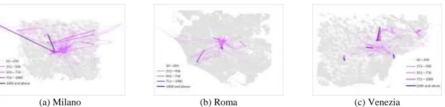
patterns. According to the travel flow volume, we can estimate the travel demand and recognize the hub of cities, so that we can make city planning and prevent the incidents.

Figure 3. Simulation results for the network.

(a) Milano (b) Roma (c) Venezia

Figure 4. The spatial distribution for all users’ trips in different Italian cities.

Conclusion

In this paper, we described the necessary steps to extract the daily origin-destination trips by purpose and time of day from Twitter data. This technique is applied to twitter data in Milano, Roma and Venezia. And this technique can be applied in other datasets with the location information.

In the stay region extracting, the grid-based algorithm is adopted. After extracting the stay region, we extract the trip of users in three cities, and visualize the trips in GIS, which clearly display the trip volume and spatial distribution. By this trip extracting, we can compute the average trip length of cities and can improve the efficiency of statistic, greatly reduce the unnecessary human consumption at the same time. We also category the trips into three types, HBW, HBO and NHB, which can help us to characterize the different features of various trip types, so that we can capture the patterns of human mobility more accurately. We analyze the distribution of user trips volume and trip length, and reveal the Zipf’s law in the human mobility. Furthermore, we prove this law is general in different cities.

Our findings can be used to recognize the patterns of human mobility more accurately. For instance, the trip length can be used in epidemic propagation model, which can characterize how long the epidemic will spread. And the trip tracks can help us to location the impacted region.

Acknowledgement

This research was financially supported by the National Science Foundation and the TIM Big Data Challenge.

References

[1] Anastasios N, Salvatore S et al. A Tale of Many Cities: Universal Patterns in Human Urban Mobility. PloS ONE, 2011, 7(5):e37027.

[2] Rozenfeld H D, Rybski D, et al. Laws of Population Growth. Proceedings of the National Academy of Sciences of the United States of America, 2008, 105(48):18702-7.

[3] Cacciapuoti A S, Calabrese F, et al. Human-mobility enabled wireless networks for emergency communications during special events. Pervasive & Mobile Computing, 2013, 9(4):472-483.

[4] Pappalardo L, Vanhoof M, et al. Estimating economic development with mobile phone data. 2016-05-30

[5] Çolak Serdar, Antonio L, González M C. Understanding congested travel in urban areas. Nature Communications, 2016, 7:10793.

[6] Blondel V D, Decuyper A, Krings G. A survey of results on mobile phone datasets analysis. Epj Data Science, 2015, 4(1):1-55.

[7] Toole J L, Herrerayaqüe C, et al. Coupling human mobility and social ties. Journal of the Royal Society Interface, 2015, 12(105):266-271.

[8] Song C, Koren T, et al. Modelling the scaling properties of human mobility. Nature Physics, 2010, 6(10):818-823.

[9] Alexander L, Jiang S, et al. Origin–destination trips by purpose and time of day inferred from mobile phone data. Transportation Research Part C Emerging Technologies, 2015, 58:240-250.

[10]Jiang S, Yang Y, et al. The TimeGeo modeling framework for urban motility without travel surveys. Proceedings of the National Academy of Sciences of the United States of America, 2016, 113(37):E5370.

[11]Pappalardo L, Simini F, et al. Returners and explorers dichotomy in human mobility. Nature Communications, 2015, 6(8166):8166.

[12]Chaintreau A, Hui P, et al. Impact of Human Mobility on Opportunistic Forwarding Algorithms. IEEE Transactions on Mobile Computing, 2007, 6(6):606-620.

[13]Fournet J, Barrat A. Contact Patterns among High School Students. PLoS ONE, 2014, 9(9):e107878.

[14]Cattuto C, Broeck W V D, et al. Dynamics of person-to-person interactions from distributed RFID sensor networks. PLoS ONE, 2010, 5(7):e11596.

[15]Rhee I, Shin M, et al. On the Levy-Walk Nature of Human Mobility// INFOCOM 2008. the Conference on Computer Communications. IEEE. IEEE Xplore, 2011:924-932.

[16]Gutiérrezroig M, Sagarra O, et al. Active and reactive behaviour in human mobility: the influence of attraction points on pedestrians. Royal Society Open Science, 2016, 3(7):33-42.

[17]Song C, Qu Z, et al. Limits of predictability in human mobility. Science, 2010, 327(5968):1018.

[19]Jiang B, Ma D, et al. Spatial Distribution of City Tweets and Their Densities. Geographical Analysis, 2016, 48(3).